Fact: Measures of center aren't enough.
To describe a distribution we need more than its center.
Example. Consider the two data sets below:
Data Set $1$:
$-1, 0, 1$
Data Set $2$:
$-1000000, 0, 1000000$
(a) What are the mean and median of Data Sets $1$ and $2?$
(b) Do the mean and median alone adequately describe these distributions?
Reminder: Averages are the most abused statistics on earth!
Example
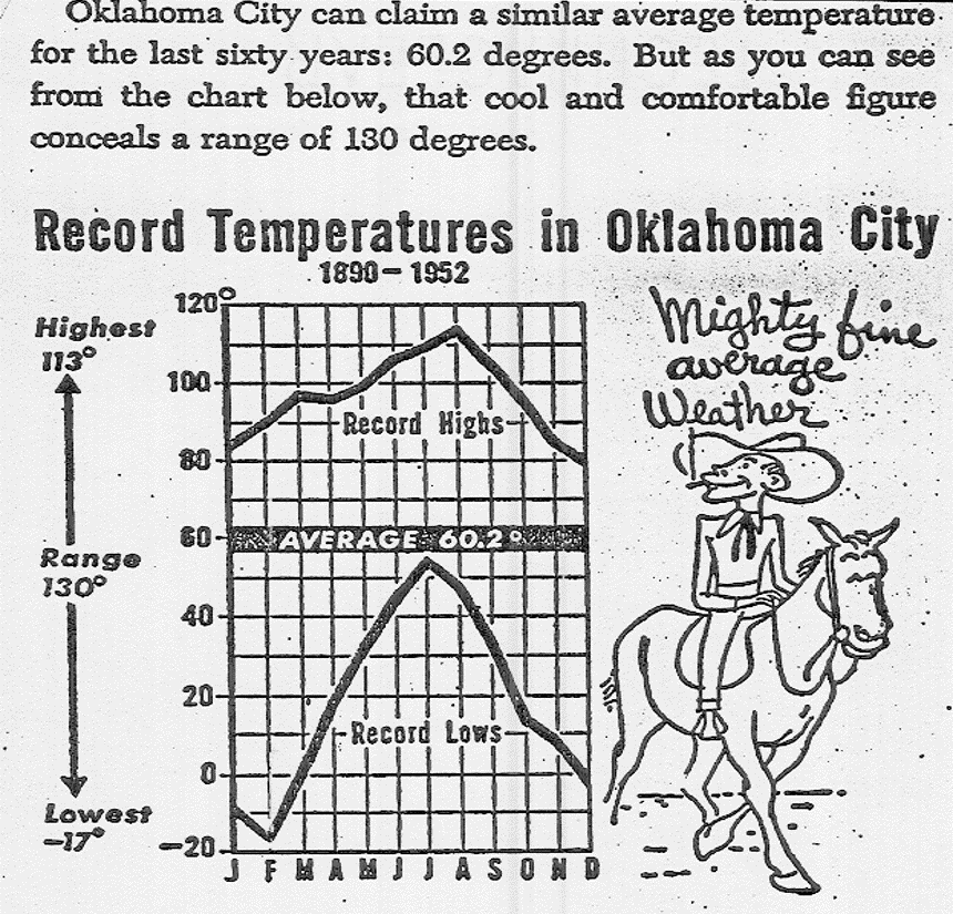
Sleazy P. Martini is a real estate agent for "Shady Real-Estate" and wants to sell you a property for which for which he says "the average yearly temperature is a lovely $60.2$ degrees!"
As a statistically savvy citizen, what questions would you ask Mr. Martini?
Quote of the Day
"A person with their feet in the freezer and their head in the oven is on the average quite comfortable."
Savvy Citizen Fact #2
Any useful numerical description of a distribution will include not only a measure of center, but also a measure of variation or spread.
A Numerical Measure of Variation: Standard Deviation
The most common measure of spread is called the standard deviation.
Standard deviation is like an "average deviation" from the mean.
Example. The standard deviation of the data set $2, 2, 2$ is $0.$
Example. The standard deviation of the data set $1, 2, 3$ is $1.$
Example. The standard deviation of the data set $0, 2, 4$ is $2.$
A Numerical Measure of Variation: Standard Deviation
Each of the data sets below have a a mean $\overline{x}=5.$
How much variation from the mean is there in this data set: $5,$ $5,$ $5,$ $5,$ $5,$ $5.$
How much variation from the mean is there in this data set: $2,$ $5,$ $4,$ $7,$ $7,$ $5.$
How much variation from the mean is there in this data set: $26,$ $-50,$ $4,$ $-40,$ $40,$ $50$
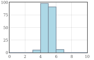
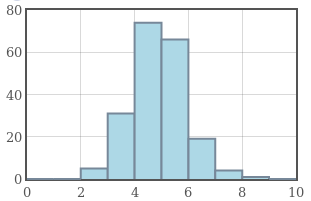
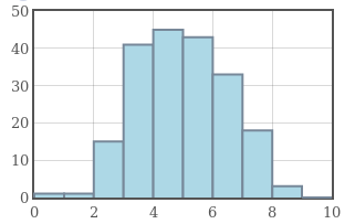
Example: The graphs below have the same mean of $5,$ but increasing standard deviation from left to right.
 |
 |
 |
Standard deviation is a measure of how concentrated a data set is around the mean.
Example: Below is a random sample of SAT Critical Reading scores.
$650,$ $490,$ $580,$ $450,$ $570$
Find the standard deviation of this data set.
The mean is $\overline{x}=548$.
$$ \begin{array}{ccc} \hline \mbox{Data Points} & \mbox{Deviations from the mean} & \mbox{Squared Deviations}\\ \hline 650 & 650 - 548 = 102 & 102^2 = 10,404 \\ \hline 490 & 490 - 548 = -58 & (-58)^2 = 3,364 \\ \hline 580 & 580 - 548 = 32 & 32^2 = 1,024 \\ \hline 450 & 450 - 548 = -98 & (-98)^2 = 9,604 \\ \hline 570 & 570 - 548 = 22 & 22^2 =484 \\ \hline & Sum=0 & Sum=24,880\\ \end{array} $$ The variance is $\displaystyle \frac{24,880}{4}=6220$.
The standard deviation is: $\sqrt{6220}\approx 78.87$.
Definitions
The variance is the "funny average" of the squared deviations from the mean.
The standard deviation is the square root of the variance.
Formula: The sample standard deviation is calculated from the following formula: $$ s=\sqrt{\frac{(x_1-\overline{x})^2+(x_2-\overline{x})^2+\cdots+(x_n-\overline{x})^2}{n-1}} =\sqrt{\frac{\displaystyle \sum (x_j-\overline{x})^2}{n-1}} $$
Fact: Fortunately, for these kinds of computations, we let technology do the grunt work for us.
For in-class exams you may use your TI-84 Calculator.
For online exams and any other written assignments you may use Holt.Blue.
Calculating the Standard Deviation from Grouped Data
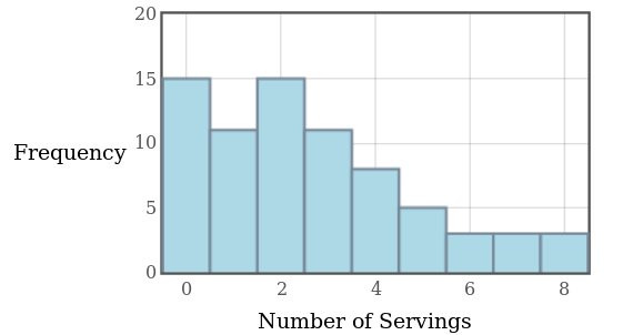
Example: The figure below is a histogram of the self-reported number of daily servings of fruit eaten for a sample of $74$ students. Calculate the standard deviation from this grouped data.
Since we know the frequency of each individual value and the mean, we can calculate the standard deviation $s$ exactly. Recently, for this data set, we calculated $\bar{x}=2.62$ servings. $$ \begin{array}{|l|l|}\hline \mbox{Servings of Fruit} & \mbox{Frequency} \\ \hline \mbox{0} & 15 \\ \hline \mbox{1} & 11 \\ \hline \mbox{2} & 15 \\ \hline \mbox{3} & 11 \\ \hline \mbox{4} & 8 \\ \hline \mbox{5} & 5 \\ \hline \mbox{6} & 3 \\ \hline \mbox{7} & 3 \\ \hline \mbox{8} & 3 \\ \hline \end{array} $$
$$ \begin{array}{|l|l|l|}\hline \mbox{Servings of Fruit} & \mbox{Frequency} & \mbox{Squared Deviations} \\ \hline \mbox{0} & 15 & (0-2.62)^2=6.86\\ \hline \mbox{1} & 11 & (1-2.62)^2=2.62\\ \hline \mbox{2} & 15 & (2-2.62)^2=0.38\\ \hline \mbox{3} & 11 & (3-2.62)^2=0.14\\ \hline \mbox{4} & 8 & (4-2.62)^2=1.90\\ \hline \mbox{5} & 5 & (5-2.62)^2=5.66\\ \hline \mbox{6} & 3 & (6-2.62)^2=11.42\\ \hline \mbox{7} & 3 & (7-2.62)^2=19.18\\ \hline \mbox{8} & 3 & (8-2.62)^2=28.94\\ \hline & & \mbox{Sum Sq. Devs}=361.08\\ \hline \end{array} $$
$$\mbox{Variance}=\frac{\mbox{Sum of Squared Deviations}}{n-1}=\frac{361.08}{73}=4.95$$ $$s=\sqrt{\mbox{Variance}}=\sqrt{4.95}\approx 2.22486$$
Calculating Standard Deviation from Grouped Data
Note: If given a histogram or frequency polygon, we can also calculate $s$.
Estimating Standard Deviation from Grouped Data
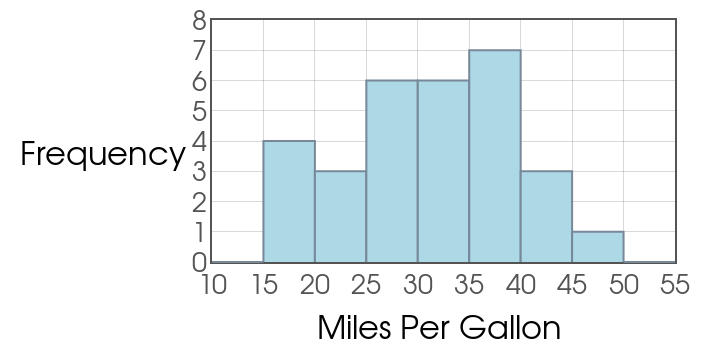
Example: Below is a frequency table of a random sample of the miles per gallon ratings of 30 cars. Estimate the standard deviation $s$ from this grouped data.
Since we DON'T know the frequency of each individual value, we estimate $s$ by using the midpoint of each interval instead of actual data values.
Recall that $\bar{x}\approx 31.17$ miles per gallon. $$ \begin{array}{|l|l|}\hline\mbox{Mileage} & \mbox{Frequency} \\ \hline \mbox{15 to 20} & 4 \\ \hline \mbox{20 to 25} & 3 \\ \hline \mbox{25 to 30} & 6 \\ \hline \mbox{30 to 35} & 6 \\ \hline \mbox{35 to 40} & 7 \\ \hline \mbox{40 to 45} & 3 \\ \hline \mbox{45 to 50} & 1 \\ \hline\end{array} $$
$$ \begin{array}{|l|l|l|}\hline\mbox{Mileage} & \mbox{Frequency} & \mbox{Squared Deviations} \\ \hline \mbox{15 to 20} & 4 & (17.5-31.17)^2=186.87\\ \hline \mbox{20 to 25} & 3 & (22.5-31.17)^2=75.17\\ \hline \mbox{25 to 30} & 6 & (27.5-31.17)^2=13.47\\ \hline \mbox{30 to 35} & 6 & (32.5-31.17)^2=1.77\\ \hline \mbox{35 to 40} & 7 & (37.5-31.17)^2=40.07\\ \hline \mbox{40 to 45} & 3 & (42.5-31.17)^2=128.37\\ \hline \mbox{45 to 50} & 1 & (47.5-31.17)^2=266.67\\ \hline & & \mbox{Sum Sq. Devs}=1996.7\\ \hline \end{array} $$
$$\mbox{Variance}=\frac{\mbox{Sum of Squared Deviations}}{n-1}=\frac{1996.7}{29}=68.83$$ $$s=\sqrt{\mbox{Variance}}=\sqrt{68.83}\approx 8.2963$$
Estimating Standard Deviation from Grouped Data
Note: If given a histogram or frequency polygon, we can also estimate standard deviation.
Application: Comparisons Between Data Sets
The heights of women aged $20$ to $29$ have a mean of $64.3$ inches and a standard deviation of $2.7$ inches. Men the same age have mean height of $69.9$ inches with standard deviation $3.1$ inches.
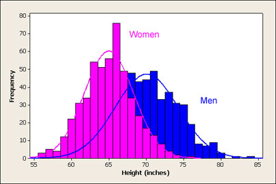
Linda Lou is $66$ inches tall, and Billy Bob is $71$ inches tall. Which person is considered taller for their group, Linda Lou, or Billy Bob?
Comparing Individuals from Different Data Sets
For an individual whose data value is $x$, compute $$z=\frac{x-\mu}{\sigma}$$ The number $z$ is the number of standard deviations from the mean.
Compare the $z$-scores for each individual.
Note: $\sigma$ is used to denote the population standard deviation.
Linda Lou's $z$-score: $\displaystyle z=\frac{x-\mu}{\sigma}=\frac{66-64.3}{2.7} \approx 0.63$
Interpretation: Linda Lou's height is $0.63$ standard deviations above the mean.
Billy Bob's $z$-score: $\displaystyle z=\frac{x-\mu}{\sigma}=\frac{71-69.9}{3.1} \approx 0.35$
Interpretation: Billy Bob's height is $0.35$ standard deviations above the mean.
Conclusion: Linda Lou would be considered taller than Billy Bob with respect to the classification of female and male.
Some More Savvy-Citizen, Golden Wisdom of the Ages
Fact: A VERY common numerical summary of a distribution is the mean $\overline{x}$ and standard deviation $s$.
Warning: This is only a good idea if your distribution is roughly a symmetric shape!
For skewed distributions it is generally better to use the five number summary:
Min, $Q1$, Median, $Q3$, Max.