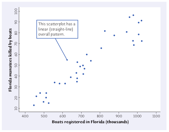
We are now going to model this data with a straight line....
Below is the manatee death versus boat registration data with a line which models the overall trend.
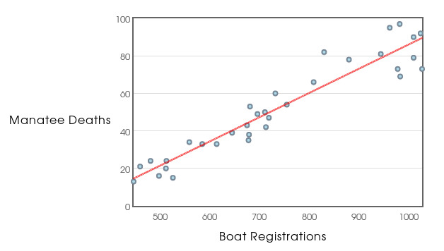
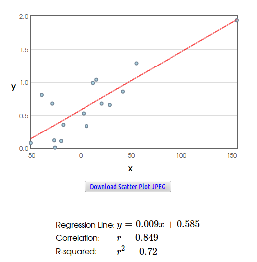
This line-of-best-fit is called a regression line.
Some Straight-Line Basics: Recall that every non-vertical straight line can be expressed in the form $y=mx+b$.
Statisticians, as well as our text, for reasons we need not yet discuss, prefer to write a generic line as $$y=a+bx.$$
Formula for the Regression Line
We can calculate the slope (written $b$ in our text) and $y$-intercept (written $a$ in our text):
the slope is $$b=r\frac{s_y}{s_x},$$
and the $y$-intercept is $$a=\bar{y}-b\bar{x}.$$
Our regression line has the form $$\hat{y}=a+bx$$
where $a$ and $b$ are given above.
The notation $\hat{y}$ is a reminder that our line gives us a prediction, or approximate guess based upon the data.
For example, the regression line for the manatee data is $\hat{y}=0.129x-43.172$. Thus, if we know in advance the number of boat registrations for the year, we can roughly predict how many manatee deaths will occur in that year.
Example: Using the regression line for the manatee data, predict the number of manatee deaths that will occur in a year with 850 boat registrations.
In this case $\hat{y}=66.418$.
Interpretation: We predict that approximately 66 manatees will die in a year in which there are 850 boat registrations.
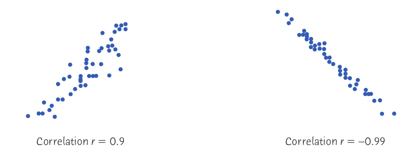
From Correlation to R-Squared: Recall that the correlation $r$ is a way of measuring the strength and direction of a linear relationship.
When we square this value, we get a more useful measure for our regression line; the percentage of the variation in the data which can be explained by our model is actually given by the value of $r^2$.
The manatee data has a correlation of $r=0.951$. The amount of variation which is explained by our regression line is $r^2=0.905$, or $90.5\%.$
Fact: The value $r^2$ is a gives us a sense of how accurate our prediction is going to be.
Low values of $r^2$ indicate a weak relationship so that our regression will yield poor predictive results.
On the other hand, high values of $r^2$ indicate a strong relationship so that our regression will yield good predictive results.
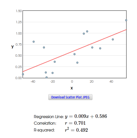
$\begin{array}{llllrrrr} r^2=0.81 & \mbox{ } & \mbox{ } & \mbox{ } & \mbox{ }& \mbox{ } & \mbox{ } & r^2=0.98\\ \end{array}$
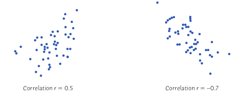 $\begin{array}{llllrrrr}
r^2=0.25 & \mbox{ } & \mbox{ } & \mbox{ } & \mbox{ }& \mbox{ } & \mbox{ } & r^2=0.49\\
\end{array}$
$\begin{array}{llllrrrr}
r^2=0.25 & \mbox{ } & \mbox{ } & \mbox{ } & \mbox{ }& \mbox{ } & \mbox{ } & r^2=0.49\\
\end{array}$
 $\begin{array}{llllrrrr}
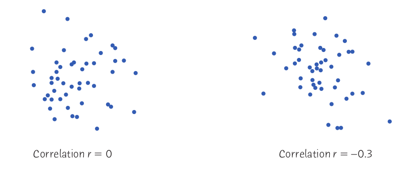
r^2=0 & \mbox{ } & \mbox{ } & \mbox{ } & \mbox{ }& \mbox{ } & \mbox{ } & r^2=0.09\\
\end{array}$
$\begin{array}{llllrrrr}
r^2=0 & \mbox{ } & \mbox{ } & \mbox{ } & \mbox{ }& \mbox{ } & \mbox{ } & r^2=0.09\\
\end{array}$
Fact: Any time you present to your reader a regression line model, you should also always report the value of $r^2$.
Residuals: A residual is the difference between a data point $y$ and the predicted value $\hat{y}$ for a given $x$.
Thus, each residual is calculated as $y-\hat{y}$ for any given value of $x$.
Below is the residual plot for the manatee data:
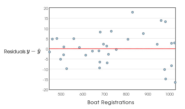
Fact: Smaller residuals mean better predictive value of the regression line.
Fact: Our regression line formula minimizes the sum of the squares of the residuals.
Influential Observations: An observation is influential for a statistical calculation ifremoving it would markedly change the result of the calculation.
The result of a statistical calculation may be of little practical use if it depends strongly on a few influential observations.
Points that are outliers in either the $x$ or the $y$ direction of a scatterplot are often influential for the correlation. Points that are outliers in the $x$ direction are often influential for the least-squares regression line.
Example: Recall the loss-aversion example we looked at in homework:
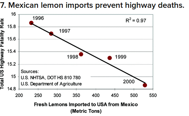
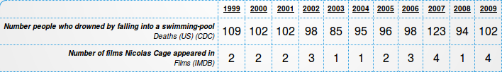
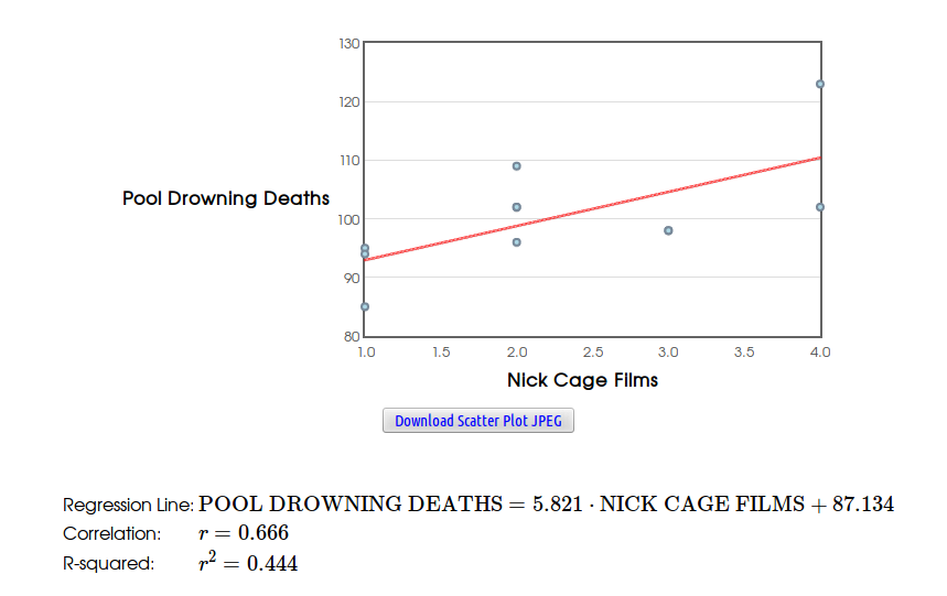
Savvy Citizen Fact #3: Correlation DOES NOT Imply Causation.
Example: Consider the relationship between lemon imports from Mexico and traffic deaths in the United States.

Beware Extrapolation: Using a statistical model to make predictions outside of a data set is called extrapolation.
Example: Suppose that you have data on a child’s growth between 3 and 8 years of age. You find a strong linear relationship between age $x$ and height $y$. If you fit a regression line to these data and use it to predict height at age 25 years, you will predict that the child will be 8 feet tall.