The Big Idea: ANOVA is a way to compare several means.
Draw an SRS from $I$ independent populations. The hypotheses of ANOVA are:
$H_0: \mu_1=\mu_2=\mu_3=\cdots=\mu_I$
$H_a: \mbox{Not all the means are equal.}$
What Does ANOVA Stand For?: ANOVA is a shortening of the phrase Analysis Of Variance.
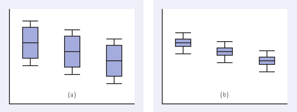
Analysis of variance is exactly what it says it is; it compares the variation between groups to the variation within groups.
If the variation between groups is considerably larger than the variation within each group, then we have evidence against the null hypothesis.
The $F$ Statistic
To compare the variation between groups to the variation within groups, we have the $F$ statistic: $$F=\frac{\mbox{variation between groups}}{\mbox{variation within groups}}$$
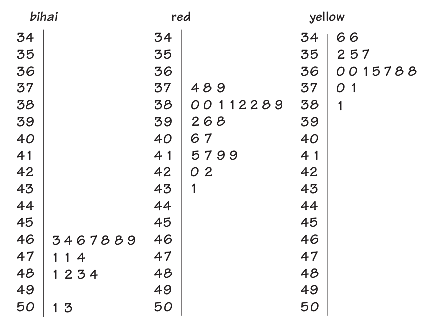
Example: Is there a relationship between varieties of the tropical flower Heliconia on the island of Dominica and the different species of hummingbirds that fertilize the flowers? Over time, the researchers believe, the lengths of the flowers and the forms of the hummingbirds’ beaks have evolved to match each other. If that is true, flower varieties fertilized by different hummingbird species should have distinct distributions of length.
Flower lengths (millimeters) for three Heliconia varieties
H. bihai: 47.12 48.07 46.75 48.34 46.81 48.15 47.12 50.26 46.67 50.12 47.43 46.34 46.44 46.64 46.94 48.36
H. caribaea red: 41.90 39.63 38.10 42.01 42.18 37.97 41.93 40.66 38.79 43.09 37.87 38.23 41.47 39.16 38.87 41.69 37.40 37.78 39.78 40.57 38.20 38.07 38.01
H. caribaea yellow: 36.78 35.17 37.02 36.82 36.52 36.66 36.11 35.68 36.03 36.03 35.45 34.57 38.13 37.10 34.63
We interupt this example to bring you a message involving terse, yet complex, mathematical statements.
Viewer discretion is advised.
Take a deep breath. You won't have to memorize these formulas. Just try to understand the big idea they encapsulate.
How to Calculate the $F$ Statistic (Part I): Let $\bar{x}$ be the sample mean for ALL individuals in the sample.
$I$ is the number of groups and $N$ is the total number of individuals in the sample.
The amount of variation BETWEEN groups is quantified as $$\mbox{MSG}=\frac{n_1(\bar{x}_1-\bar{x})^2+n_2(\bar{x}_2-\bar{x})^2+\cdots+n_I(\bar{x}_I-\bar{x})^2}{I-1}$$ This value is known as the Mean Square for Groups or MSG.
The degrees of freedom for this calculation is $I-1$.
How to Calculate the $F$ Statistic (Part II): $I$ is the number of groups and $N$ is the total number of individuals in the sample.
The amount of variation WITHIN groups is quantified as $$\mbox{MSE}=\frac{(n_1-1)s_1^2+(n_2-1)s_2^2+\cdots+(n_I-1)s_I^2}{N-I}$$ This value is known as the Mean Square for Error or MSE.
The degrees of freedom for this calculation is $N-I$.
How to Calculate the $F$ Statistic (Part III: The Final Chapter)
The $F$ statistic with $I-1$ degrees of freedom in the numerator and $N-I$ degrees of freedom in the denominator is:
$$F=\frac{\mbox{MSG}}{\mbox{MSE}}$$
The Big Deal
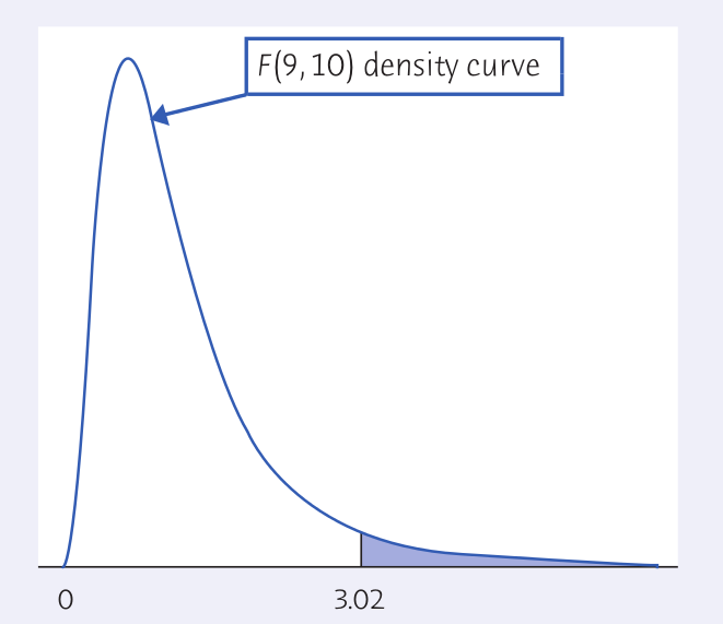
If the null hypothesis is true, that is, if $\mu_1=\mu_2=\mu_3=\cdots=\mu_I$, then the $F$ statistic follows an $F$ distribution with $I-1$ degrees of freedom in the numerator and $N-I$ degrees of freedom in the denominator.
Example: Below is the density curve for the $F$ distribution having 9 degrees of freedom in the numerator and 10 degrees of freedom in the denominator.
Now Back to Our Regularly Scheduled Example...
Flower lengths (millimeters) for three Heliconia varieties
H. bihai: 47.12 48.07 46.75 48.34 46.81 48.15 47.12 50.26 46.67 50.12 47.43 46.34 46.44 46.64 46.94 48.36
H. caribaea red: 41.90 39.63 38.10 42.01 42.18 37.97 41.93 40.66 38.79 43.09 37.87 38.23 41.47 39.16 38.87 41.69 37.40 37.78 39.78 40.57 38.20 38.07 38.01
H. caribaea yellow: 36.78 35.17 37.02 36.82 36.52 36.66 36.11 35.68 36.03 36.03 35.45 34.57 38.13 37.10 34.63
Pop Quiz: What is $I$? What is $N$?
When You Assume...
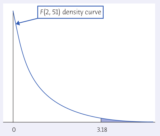
If the null hypothesis is true, that is if all the means are equal, then the $F$ statistic follows an $F$ distribution with $I-1=3-1=2$ degrees of freedom in the numerator and $N-I=54-3=51$ degrees of freedom in the denominator.
Below is the density curve for $F(2,51)$ with the critical value 3.18 for the significance level $\alpha=0.05$.
Finally We Can Get Some Results!
Let's run an ANOVA on our data!
English Language Conclusion?
The Fine Print: Conditions for Inference
1) ANOVA requires independent SRSs from each group. If you don't have this, any analysis is essentially worthless.
2) ANOVA assumes that each population is normally distributed. Fortunately, ANOVA is robust enough to withstand non-extreme deviations from normally thanks to ______________.
3) ANOVA assumes that all population standard deviations $\sigma$ are equal.
Big Question: Is ANOVA robust against violations of assumption 3?
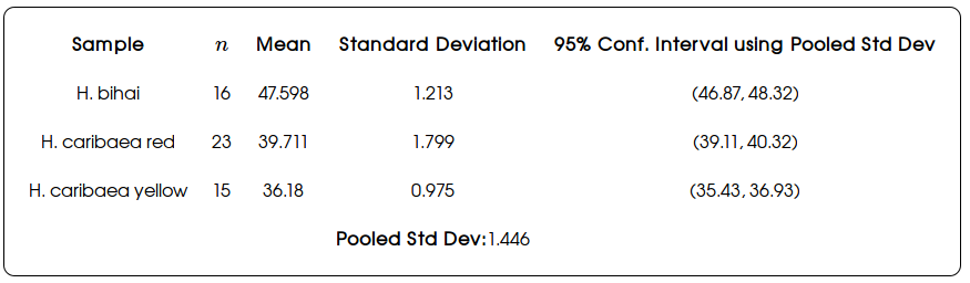
Checking Standard Deviations
The results of the ANOVA $F$ test are approximately correct when the largest sample standard deviation is no more than twice as large as the smallest sample standard deviation.
From Our Example : Do our sample standard deviations satisfy this rule?
A Recommendation
ANOVA is not too sensitive to violations of assumption 3, especially when all samples have the same or similar sizes and no sample is very small. When designing a study, try to take samples of about the same size from all the groups you want to compare.