The Big Idea: The Chi-Square Test is a way to determine if two categorical variables are related to each other.
Example: The University of Chicago’s General Social Survey (GSS) is the nation’s most important social science sample survey. The GSS asked a random sample of adults their opinion about whether astrology is very scientific, sort of scientific, or not at all scientific.
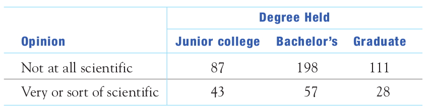
Question: Which two categorical variables does this table compare?
A Probabilistic Aside: Independent Events.
A Fun Question: If we flip a coin, and it comes up heads, does that give us any information about the outcome of the next flip?
Answer:
Another Fun Question: Suppose we pluck a random person and consider the probability that they voted for Candidate A (Libelous Party) or Candidate B (Preservative Party), does knowing this person's socioeconomic status change the probability of one outcome over the other?
Answer:
A Definition: Two events $A$ and $B$ are independent if the outcome of one has no effect on the probability of the other. In fancy mathematical notation we write $$P(A|B)=P(A) \,\,\,\,\mbox{ and }\,\,\,\, P(B|A)=P(B).$$ Example: Coin tosses, dice rolls, and other such things are independent events.
Example: Political affiliation and socioeconomic status, on the other hand, are harder to determine whether or not they are independent. Enter the Chi-Square Test!
Back to Our Example: Faith in Astrology versus Level of Education
$H_0:$ Faith in Astrology and Level of Education are independent.
$H_a:$ Faith in Astrology and Level of Education are NOT independent.
Thought Experiment: Let's suppose that : Faith in Astrology and Level of Education are independent.
Looking at our two-way table, how many people would we expect to fall into the category of "not scientific" with a "junior college" level of education if these two categories are independent?
Then using laws of probability $$\frac{P(\mbox{not scientific AND junior college})}{P(\mbox{junior college})}=P(\mbox{not scientific})$$ so that $$P(\mbox{not scientific AND junior college})=P(\mbox{not scientific}) \cdot P(\mbox{junior college})$$ In terms of our table, this means $$\frac{\mbox{Expected Count of Not Scientific AND Junior College}}{524}=\frac{396}{524} \cdot \frac{130}{524}$$ After even more algebraic monkeyshines, we get...
$$\mbox{Expected Count of Not Scientific AND Junior College}=\frac{396 \cdot 130}{524}$$
In general, the expected count for a given entry in our table is $$\mbox{Expected Count}=\frac{\mbox{row total $\times$ column total}}{\mbox{table total}}$$
Now we saw that $$\mbox{Expected Count of Not Scientific AND Junior College}=\frac{396 \cdot 130}{524}$$ or $$\mbox{Expected Count of Not Scientific AND Junior College}=98.24$$ How does this compare to what we actually observed?
The observed count in our table is 87.
Is this a big difference?
The Chi-Square Test: The Big Idea
For every entry in our two-way table, we calculate the expected count assuming independence.
If these expected counts differ greatly from what we actually observe, then we have evidence that the two categorical variables are not independent.
The Chi-Square Test: The Details
The chi-square statistic is a measure of how far the observed counts in a two-way table are from the expected counts. The formula for the statistic is $$\chi^2=\sum \frac{(\mbox{observed count$-$expected count})^2}{\mbox{expected count}}$$ If the expected counts differ greatly from what we actually observe, the chi-square statistic is large.
On the other hand, if the expected counts are close to what we actually observe, then chi-square is small.
Question: What kind of distribution does the $\chi^2$-statistic follow?
Answer: A $\chi^2$ distribution. DUH!
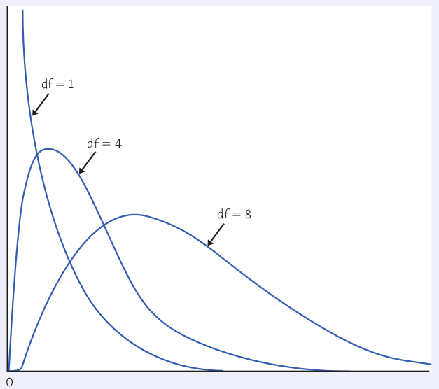
The Chi-Square Distributions
The chi-square distributions are a family of distributions that take only positive values and are skewed to the right. A specific chi-square distribution is specified by giving its degrees of freedom.
The chi-square test for a two-way table with $r$ rows and $c$ columns uses critical values from the chi-square distribution with $(r - 1)(c - 1)$ degrees of freedom. The $p$-value is the area under the density curve of this chi-square distribution to the right of the value of test statistic.
Back to Our Original Example...Finally!
Are faith in astrology and level of education related?
Let's find out by running a Chi-Square Test on our original example using holt.blue!
The Fine Print: Conditions For Inference
The results of a chi-square test may be trusted when:
- no more than 20% of the expected counts are less than 5 AND
- all individual expected counts are 1 or greater.
Of course, our sample must also be a(n) _____________________!!!
One More Detail: Every individual in your sample may belong to only one cell in your table. Otherwise, chi-square is not the right test.
Another Use of $\chi^2$: Goodness of Fit
Recall: Sleazy P. Martini was convicted of gaming fraud with his crooked die. Recall that the court used a significance level of $\alpha=0.01$. Sleazy P.'s lawyer decided to look at the data again.
Are there grounds for an appeal?
Looking again at the data:
5 1 6 5 5 6 4 5 4 3 4 3 5 6 2 3 2 4 6 2 6 6 2 6 6 2 2 2 4 2 6 5 5 2 2 4 6 6 3 6 1 4 3 3 3 4 6 4 3 2 6 6 6 6 3 4 3 5 1 6 6 5 2 5 2 1 3 1 6 3 4 3 5 6 3 6 6 5 6 4 3 4 1 3 6 4 2 6 5 3 2 6 2 5 5 5 5 5 1 4
The observed counts for the 100 recorded rolls are $$ \begin{array}{c|c|c|c|c|c|c} \hline \mbox{outcome} & 1 & 2 & 3 & 4 & 5 & 6 \\\hline \mbox{observed count} & 7 & 16 & 17 & 15 & 18 & 27 \\\hline \end{array} $$ The expected counts assuming a fair die are $$ \begin{array}{c|c|c|c|c|c} \hline \mbox{outcome} & 1 & 2 & 3 & 4 & 5 & 6 \\\hline \mbox{expected count} & 16.7 & 16.7 & 16.7 & 16.7 & 16.7 & 16.7 \\\hline \end{array} $$
We again compute the chi-square statistic $$\chi^2=\sum \frac{(\mbox{observed count$-$expected count})^2}{\mbox{expected count}}$$ which in this case follows a chi-square distribution with 5 degrees of freedom.
Let's run the analysis on holt.blue!
The $\chi^2$ Goodness of Fit Test
A categorical variable has $k$ possible outcomes, with probabilities $p_1$, $p_2$, $p_3$, . . . , $p_k$. That is, $p_i$ is the probability of the $i$th outcome. We have $n$ independent observations from this categorical variable.
To test the null hypothesis that the probabilities have specified values $H_0: p_1 = p_{10}, p_2 = p_{20}, \ldots , p_k = p_{k0}$ find the expected count for the $i$th possible outcome as $np_{i0}$ and use the chi-square statistic $$\chi^2=\sum \frac{(\mbox{observed count$-$expected count})^2}{\mbox{expected count}}$$ The $p$-value is the area to the right of $\chi^2$ under the density curve of the chi-square distribution with $k - 1$ degrees of freedom.