Example: A surprising number of young adults (ages 19 to 25) still live in their parents’ home. A random sample by the National Institutes of Health included 2253 men and 2629 women in this age group. The survey found that 986 of the men and 923 of the women lived with their parents.
Comparing Two Proportions
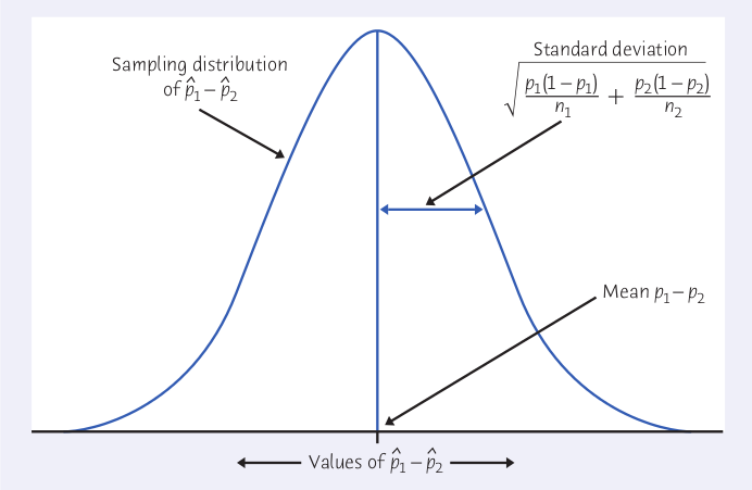
The proportion for young men is $$\hat{p}_1=\frac{986}{2253}=0.4376$$ and the proportion for young women is $$\hat{p}_2=\frac{923}{2629}=0.3511$$ Is this good evidence that different proportions of young men and young women live with their parents?
Pop Quiz: What kind of distribution does the quantity $\hat{p}_1-\hat{p}_2$ follow?
Hint: Use your newly acquired statistically savvy intuition. ;)
How to Estimate $p_1-p_2$
Large-Sample Confidence Interval
Draw an SRS of size $n_1$ from a large population having proportion $p_1$ of successes and draw an independent SRS of size $n_2$ from another large population having proportion $p_2$ of successes. When $n_1$ and $n_2$ are large, an approximate level $C$ confidence interval for $p_1 - p_2$ is $$(p_1-p_2) \pm z^* \sqrt{\frac{\hat{p}_1(1-\hat{p_1})}{n_1}+\frac{\hat{p}_2(1-\hat{p_2})}{n_2}}$$ Use this interval only when the numbers of successes and failures are each 10 or more in both samples.
Returning to Our Example...
Recall that proportion for young men living with their parents is $\hat{p}_1=0.4376$ and the proportion for young women living with their parents is $\hat{p}_2=0.3511$.
Lets calculate a confidence interval for $p_1-p_2$. (Important! Are the conditions met for using this interval?)
Any guesses before we do?
Large-Sample 95% Confidence Interval $$(0.4376-0.3511) \pm 1.96 \sqrt{\frac{0.4376(1-0.4376)}{2253}+\frac{0.3511(1-0.3511)}{2629}}$$ Simplifying we get $$(0.059,0.114)$$ What is our conclusion?
Don't forget, you can always use holt.blue
Problems... Again!
One big problem with these techniques is that they give accurate results only when the sample size is large.
Another problem is with small sample sizes, the counts of successes and failures may be too small, rendering the use of these techniques untrustworthy.
Question: Who remembers how we dealt with this problem for a single proportion?
The "Plus Four" Confidence Interval.
Suppose you take two samples from two distinct populations respectively of size $n_1$ with $m_1$ successes and size $n_2$ with $m_2$ successes. Instead of computing $\hat{p}_1=\frac{m_1}{n_1}$ and $\hat{p}_2=\frac{m_2}{n_2}$, compute the "plus four" estimates $$\tilde{p}_1=\frac{m_1+1}{n_1+2} \mbox{ and } \tilde{p}_2=\frac{m_2+1}{n_2+2}$$ The two-sample "plus four" confidence interval is $$(\tilde{p}_1-\tilde{p}_2) \pm z^* \sqrt{\frac{\tilde{p}_1(1-\tilde{p_1})}{n_1+2}+\frac{\tilde{p}_2(1-\tilde{p_2})}{n_2+2}}$$ Use this interval when the sample size is at least 5 in each group, with any counts of successes and failures.
Example: Broken crackers.
We don’t like to find broken crackers when we open the package. How can makers reduce breaking? One idea is to microwave the crackers for 30 seconds right after baking them. Breaks start as hairline cracks called “checking.” Assign 65 newly baked crackers to the microwave and another 65 to a control group that is not microwaved. After one day, none of the microwave group and 16 of the control group show checking. Give the 95% plus four confidence interval for the amount by which microwaving reduces the proportion of checking.
Broken Crackers Continued
Our "plus four" estimates are $\tilde{p}_1=\frac{0+1}{65+2}=0.015$ and $\tilde{p}_2=\frac{16+1}{65+2}=0.254$.
The 90% confidence interval is then $$(0.015-0.254) \pm 1.645 \sqrt{\frac{0.015(1-0.015)}{65+2}+\frac{0.254(1-0.254)}{65+2}},$$ or $(-0.329, -0.148)$
What is our conclusion?
Tests of Significance
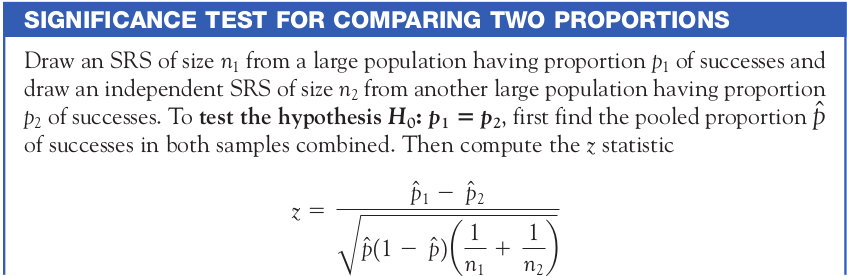
Note: The pooled proportion $\hat{p}$ is the total number of successes divided by the sum of the sample sizes. That is, $$\hat{p}=\frac{\mbox{number of successes in both samples combined}}{\mbox{number of individuals in both samples combined}}$$
Adult Children Living with Parents Revisited
Recall that a surprising number of young adults (ages 19 to 25) still live in their parents’ home. A random sample by the National Institutes of Health included 2253 men and 2629 women in this age group. The survey found that 986 of the men and 923 of the women lived with their parents. Is this good evidence that different proportions of young men and young women live with their parents?
Lets perform a test of significance for $p_1-p_2$. (Important! Are the conditions met for using this test?)
Any guesses before we do?
First Step: State Hypotheses
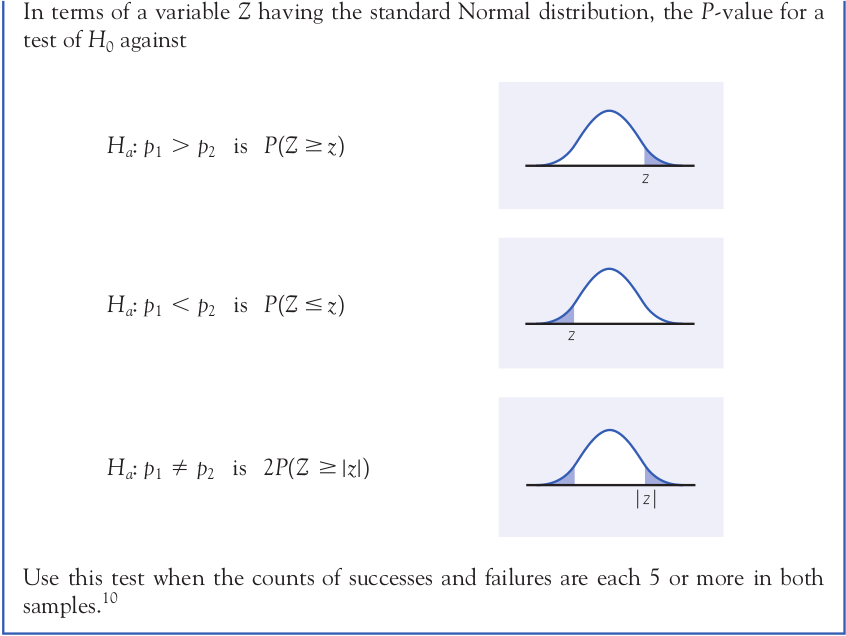
What are our hypotheses if we want to test that there is simply a difference in both populations?
Second Step: Compute Test Statistic
The proportion for young men is $\hat{p}_1=\frac{986}{2253}=0.4376.$
The proportion for young women is $\hat{p}_2=\frac{923}{2629}=0.3511.$
The pooled proportion is $\hat{p}=\frac{986+923}{2253+2629}=0.3910.$
The $z$-statistic is $$z=\frac{0.4376-0.3511}{\sqrt{0.3910(1-0.3910)(\frac{1}{2253}+\frac{1}{2629})}}$$
Third Step: Compute $p$-value
$z=6.174$.
$p=$
Fourth Step: State Your Conclusion
With a very small $p$-value, there is very strong evidence against the null hypothesis.
We conclude, therefore, that there the two population proportions are NOT the same.