Question: What are the two types of statistical inference we have studied so far?
Recall
- Confidence Intervals: $\bar{x} \pm z^*\frac{\sigma}{\sqrt{n}}$
- Tests of Significance: the $z$ statistic $z=\frac{\bar{x}-\mu}{\sigma/\sqrt{n}}$
Question: What was a major drawback of the $z$ procedures?
The $t$ Procedures
The $t$-procedures don't require that we know $\sigma$.
Instead of the population standard deviation $\sigma$, we use the sample standard deviation $s$.
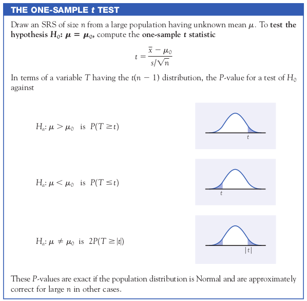
The value $$t=\frac{\bar{x}-\mu}{s/\sqrt{n}}$$ follows a $t$-distribution.
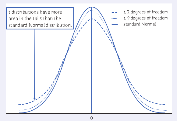
The $t$ Distributions: Draw an SRS from a normally distributed population and compute $t=\frac{\bar{x}-\mu}{s/\sqrt{n}}$. Then $t$ follows the $t$ distribution with $n-1$ degrees of freedom.
The Big Deal: We can now fully practice inference for a population mean.
Critical Values of the $t$ Distribution
But before we move on to the serious business of estimating population means...
Question: What is $z^*$?
Critical Values of the $t$ Distribution
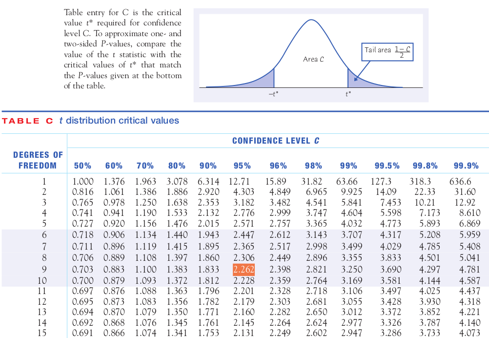
$t^*$ is the value of $t$ on a $t$ Distribution which gives us the desired level of confidence.
Example: Calculate $t^*$ for 95% confidence with sample size 10 (i.e., 9 degrees of freedom).
Method 1: Table C in Your Text.
Method 2: Software.
This means either purchasing a statistical software package, or using holt.blue.
You also have the option of using your TI-84 Calculator.
We are now ready to embark upon our inferential journey!
The One-Sample $t$ Confidence Interval
Draw an SRS of size $n$ from a population with unknown mean $\mu$. A $C\%$ confidence interval for $\mu$ is $$\bar{x} \pm t^* \frac{s}{\sqrt{n}}$$ where $t^*$ is the critical value of the $t$ distribution with $n-1$ degrees of freedom.
Example: Recall Sleazy P.'s Loaded Die Data.
5 1 6 5 5 6 4 5 4 3 4 3 5 6 2 3 2 4 6 2 6 6 2 6 6 2 2 2 4 2 6 5 5 2 2 4 6 6 3 6 1 4 3 3 3 4 6 4 3 2 6 6 6 6 3 4 3 5 1 6 6 5 2 5 2 1 3 1 6 3 4 3 5 6 3 6 6 5 6 4 3 4 1 3 6 4 2 6 5 3 2 6 2 5 5 5 5 5 1 4
The mean of the above data is $\bar{x}=4.02$ and the sample standard deviation is $s=1.651$.
Use Table C to calculate a 95% confidence interval for the true mean of Sleazy P.'s loaded die.
Example: Use holt.blue to calculate a 95% confidence interval for the Loaded Die Data.
The Fine Print: When is it appropriate to use the $t$-procedures?
Except in the case of small samples, the condition that the data are an SRS from the population of interest is more important than the condition that the population distribution is Normal.
Sample size less than 15: Use $t$ procedures if the data appear close to Normal (roughly symmetric, single peak, no outliers). If the data are clearly skewed or if outliers are present, do not use $t$.
Sample size at least 15: The $t$ procedures can be used except in the presence of outliers or strong skewness.
Large samples: The $t$ procedures can be used even for clearly skewed distributions when the sample is large, roughly $n \geq 40.$
Robustness of the $t$ Procedures
Vocab: A statistical procedure is called robust if violations of its initial assumptions cause little change in the results (i.e., $p$-values, margins of error, and so forth.)
Example: Mr. Holt owns a fuel efficient car (this is true). And Mr. Holt really collected data on the mileage per gallon on a recent trip to Southern California. The following mileages/gallon on the highway were recorded at each fill-up:
40.71 38.99 36.88 33.05 37.43
Is it safe to use the $t$-procedures with these data? If so, calculate a 99% confidence interval using
- Table C ($\bar{x}=37.412$ and $s=2.8582$)
- holt.blue
- Your TI-84 Calculator.
Example: The composition of the earth's atmosphere may have changed over time. To try to discover the nature of the atmosphere long ago, we can examine the gas in bubbles inside ancient amber. The trapped gases should be a sample of the atmosphere at the time the amber was formed. Amber from the late Cretaceous era (75 to 95 million years ago) give these percents of nitrogen:
63.4 65.0 64.4 63.3 54.8 64.5 60.8 49.1 51.0
Assume that these observations are an SRS. With a small sample size, we wonder if it's safe to use the $t$-procedures with these data? If so, calculate a 90% confidence interval to estimate the mean percent of nitrogen in ancient air.
Now we know how to estimate an unknown population mean in a realistic way.
Congratulations!
What is the other type on inference we are going to talk about next?
Tests of Significance: The One-Sample $t$-Test
Example: Mr. Holt owns a fuel efficient car (this is true). And Mr. Holt really collected data on the mileage per gallon on a recent trip to Southern California. The following mileages/gallon on the highway were recorded at each fill-up:
40.71 38.99 36.88 33.05 37.43
The true average highway fuel efficiency of the make and model of Mr. Holt's car is 34 miles per gallon. Does Mr. Holt have good evidence that his car is actually more fuel efficient than the average? Carry out a One-Sample $t$-test to find out. Use a significance level of $\alpha=0.05.$
Step 1: State the null and alternative hypotheses.
Step 2: Calculate the $t$-test statistic. (Recall: $\bar{x}=37.412$ and $s=2.8582$.)
Step 3: Get $p$-value. (With Table C, we can only say that $p$ is above or below $\alpha=0.05$.)
Step 4: State conclusion.
Example: Use holt.blue to perform a One-Sample $t$-Test using a significance level of $\alpha=0.05$.
Sleazy P. on Trial Again: Do the die-toss data given above give good evidence that Sleazy P. loaded the die? (That is, is there evidence that the mean of the die is not equal to 3.5?) To find out, we perform a One-Sample $t$-Test. Since Sleazy P.'s freedom is on the line, we'll use a stricter significance level of $\alpha=0.01$.
Although we will use software, in this case holt.blue, we will still use the four-step process outlined above.
Example: To investigate water quality in 2010, the Columbus Dispatch took water samples at 20 Ohio State Park swimming areas. They were taken to laboratories and tested for fecal coliform. An unsafe level of fecal coliform means there’s a higher risk that a swimmer will become ill. Ohio considers it unsafe if a 100-milliliter sample of water contains more than 400 coliform bacteria. Here are the fecal coliform levels:
160 40 3000 2200 2800 80 2000 15 80 2000 2000 2000 1500 2600 400 600 150 1000 500 1500
Do you think it's safe to use the $t$-procedures with these data?
Are these data good evidence that, on average, the fecal coliform levels in these swimming areas were unsafe?
With the $t$-procedures firmly in hand, we can now compare treatments in an experiment.
Recall: In a matched pairs design either
1) subjects are matched in pairs and each treatment is given to one subject in each pair.
OR
2) before-and-after observations on the same subjects are compared.
Matched Pairs $t$-Procedure: Use software.
To compare the responses to the two treatments in a matched pairs design:
1) find the difference between the responses within each pair
2) then apply the one-sample $t$-procedures to these differences.
$H_0: \mu=0$
$H_a$: either $\mu > 0$, $\mu < 0$, or $\mu \neq 0$, depending on test.
Example: Does a football filled with helium travel farther than one filled with ordinary air? To test this, the Columbus Dispatch conducted a study. Two identical footballs, one filled with helium and one filled with ordinary air, were used. A trial consisted of kicking both footballs in a random order. The kicker did not know which football (the helium-filled or the air-filled football) he was kicking.
Here are the data for the 39 trials, in yards that the footballs traveled.
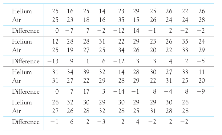
The differences (helium minus air) is the response variable.
The differences (helium minus air) are:
0 -7 7 -2 -12 14 -1 2 -2 -2 -13 9 1 6 -12 3 3 4 2 -5 0 7 17 3 -14 -1 8 -4 8 -9 -1 6 2 -3 2 4 -2 2 -2
Is it reasonable to use the $t$-procedures?
If your conclusion in part is 'Yes," do the data give convincing evidence that the helium-filled football travels farther than the air-filled football?