Sleazy P. Martini Goes On Trial
Sleazy P. Martini is up to his old tricks again, throwing dice on the wharf and winning lots of bets. You (an observer with statistical knowledge) suspect that Sleazy P. is pulling some shenanigans. That is, you suspect the die he is using is loaded.
Question: How do you prove this?
Sleazy P. Martini Goes On Trial
Partial Answer: You collect data.
You start writing down the result of each roll of Sleazy P.'s die, and record the following data:
5 1 6 5 5 6 4 5 4 3 4 3 5 6 2 3 2 4 6 2 6 6 2 6 6 2 2 2 4 2 6 5 5 2 2 4 6 6 3 6 1 4 3 3 3 4 6 4 3 2 6 6 6 6 3 4 3 5 1 6 6 5 2 5 2 1 3 1 6 3 4 3 5 6 3 6 6 5 6 4 3 4 1 3 6 4 2 6 5 3 2 6 2 5 5 5 5 5 1 4
The sample mean of the above data is $\overline{x}=4.02.$
Is this evidence that Sleazy P. has loaded the die?
The Sampling Disribution
If Sleazy P. is innocent, the sampling distributions should be very close to $$N(3.5,0.171).$$ Assuming that Sleazy P. is innocent, what is the probability of seeing the sample mean we recorded?
Busted! Sleazy P. Goes to Jail
Assuming that Sleazy P. is innocent, the chances of observing a sample mean as far from 3.5 as $\bar{x}=4.02$ over 100 rolls is 0.0024.
This is very strong evidence that he is not innocent, but that he actually loaded the die.
Hypothesis Testing
We just performed a hypothesis test.
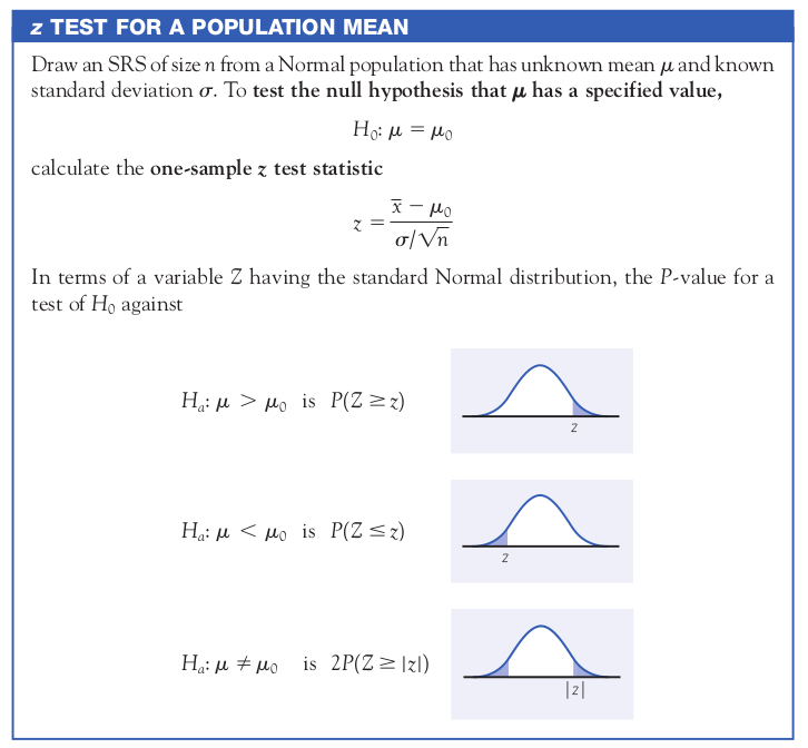
The null hypothesis is that Sleazy P. is that innocent and that the true mean of his die is 3.5. This is denoted as $$H_0: \mu=3.5.$$ The alternative hypothesis is that Sleazy P. is guilty, and really did load the die, altering the fair-die mean of 3.5. We denote this as $$H_a: \mu \neq 3.5$$
Hypothesis Testing
We saw that the probability that Sleazy P. is innocent given the sample mean we recorded was 0.0024.
We computed a test statistic: $$z=\frac{\bar{x}-\mu}{\sigma/\sqrt{n}}=\frac{4.02-3.5}{1.71/\sqrt{100}}=3.04$$ The probability of observing a test statistic AS EXTREME OR MORE EXTREME than 3.04 is 0.0024.
The value 0.0024 is called the $p$-value of the test.
Vocab
We say that the result of hypothesis test is statistically significant if the $p$-value falls below a certain threshold.
Common thresholds are $\alpha=0.05$ and $\alpha=0.01.$
In this case, we say that a test is significant at the level of $\alpha$ when $p<\alpha.$
In the case of statistical significance ($p<\alpha$), we reject the null hypothesis.
Another way to say it:
When the $p$-value's low, $H_0$ has got to go!
OR...
If the $p$-value's low, reject the  !
!
!
In Sleazy P's case, at the level of significance $\alpha=0.01$, there is statistically significant evidence that he loaded the die since $p=0.0024<0.01.$
Note: The result is significant at the 0.05 level too.
Consumer Advocacy: Sleazy P. Gets out of Jail
After serving his sentence, Sleazy P. Martini is now rehabilitated and ready to enter society as a soft drink manufacturer.
Sleazy P. has created a new brand of cola called "Sleazy P.'s Easy Peazy."
Now, a 12 fl oz can of soda should contain 355 ml of product, but you (the statistically savvy citizen) notice that in general, there seems on average to be less.
Hmmmmm.... Is Sleazy P. up to his old tricks AGAIN!?
Big Question: How do we find out?
Big Answer: Gather data and perform a hypothesis test.
Because 355 ml is printed on the can, we know the true mean $\mu$ should be a little bigger than 355 to prevent underfilling.
After a little research, we learn from various soft drink manufacturers that, in fact, the amount should vary according to a normal distribution with mean $\mu = 355.2$ ml and standard deviation $\sigma = 0.5$ ml.
Next, we begin collecting data...
The Data: Taking a simple random sample from around the country, we procured 40 cans of Sleazy P.'s Easy Peazy. Here is the data.
355.1713 354.7491 354.4016 355.1750 355.3161 354.5041 354.1384 354.4409 355.2909 355.1111 353.9682 354.3925 355.3109 355.1482 354.9777 354.9706 355.5698 356.0415 354.8885 356.2408 354.5592 354.9683 355.8299 354.8858 354.1747 354.8914 355.1179 354.4572 355.2101 354.0452 354.0947 355.4796 354.7673 354.9906 355.1146 355.6792 355.7509 355.1079 354.9283 355.6420
The Hypothesis Test
$$H_0: \mu=355.2$$ $$H_a: \mu<355.2$$
From our data we get $\overline{x}=354.98755.$
Using $\sigma=0.5$ we compute the $z$ statistic:
$$z=\frac{\bar{x}-\mu}{\sigma/\sqrt{n}}=\frac{354.99-355.2}{0.5/\sqrt{40}}=−2.66$$
The $p$-value for this test statistic is $p=.0039.$
Interpretation
Given that the null hypothesis ($H_0: \mu=355.2$) is true, the chances of seeing a test statistic of $z=-2.66$ OR LESS is 0.0039. That is, $p=0.0039.$
At the $\alpha=0.01$ level of significance, we reject the null hypothesis.
Conclusion: Reject $H_0.$ That is, Sleazy P. is underfilling. Thus, we can still count on Sleazy P. to be a shady wheeler-dealer.
The General Hypothesis Test
The General Hypothesis Test
When you perform a hypothesis test, you need to:
Step 1: State your hypotheses: $H_0$ and $H_a.$
Step 2: Compute the test statistic (in this case, the $z$-statistic).
Step 3: Determine your $p$-value.
Step 4: State your conclusion (keep or reject $H_0$). If your $p$-value falls below $\alpha$, then we reject $H_0$. Otherwise, we keep $H_0$. Also, summarize the conclusion using the language of the problem situation.