Probability: The Big Idea
A probability is a long term proportion of a certain outcome.
Example: Toss a coin. What is the probability of getting heads or tails?
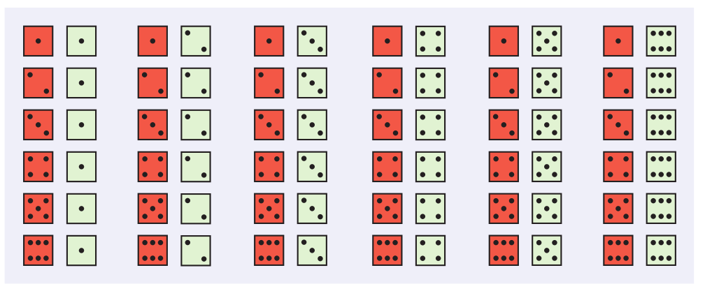
Example: Roll a pair of dice and take the sum of their faces. What is the probability of rolling a 3?
Below is a table of all possible rolls.
Probability Vocab
The sample space $S$ of a random phenomenon is the set of all possible outcomes.
An event is an outcome or a set of outcomes of a random phenomenon. That is, an event is a subset of the sample space.
A probability model is a mathematical description of a random phenomenon consisting of two parts: a sample space S and a way of assigning probabilities to events.
For the dice pair rolling example, the sample space $S$ is the collections of all possible rolls:
The event "roll a 3" is the subset of all pairs which sum to 3
{
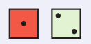 ,
,
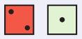 }
}
,
}
The entire probability model for the dice pair example is.
$$ \begin{array}{c} P(\mbox{rolling a 2})=1/36\\ P(\mbox{rolling a 3})=2/36\\ P(\mbox{rolling a 4})=3/36\\ P(\mbox{rolling a 5})=4/36\\ P(\mbox{rolling a 6})=5/36\\ P(\mbox{rolling a 7})=6/36\\ P(\mbox{rolling a 8})=5/36\\ P(\mbox{rolling a 9})=4/36\\ P(\mbox{rolling a 10})=3/36\\ P(\mbox{rolling a 11})=2/36\\ P(\mbox{rolling a 12})=1/36\\ \end{array} $$
Exercise: Let roll a pair of dice and see for ourselves how often we "roll a 3."
The Ground Rules of Probability: Any valid probability model must obey the following rules.
Rule #1 The probability of any event $A$ is between 0 and 1. That is, $0\leq P(A) \leq 1$.
Rule #2 The probability of the sample space is always 1. That is $P(S)=1$.
Rule #3 The probability of an event $A$ NOT occurring is $1-P(A)$. That is, $P(A^c)=1-P(A)$.
Rule #4 If the events $A$ and $B$ have no outcomes in common, then $P(A \mbox{ or } B)=P(A)+P(B)$
Another Fun Example: Benford's Law.
The first digits of numbers in legitimate records often follow a model known as Benford’s law. Call the first digit of a randomly chosen record $X.$ Benford’s law gives this probability model for $X$:
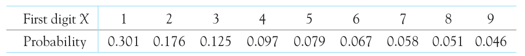
What is the probability that the first number is not 1? (Hint: Use Rule #3.)
What is the probability that the first number is a 3 or 4? (Hint: Use Rule #4.)
Classifying Probability Models: There are three kinds of probability models we need to know about.
1. Finite Probability Models. The sample space is finite. Examples: Tossing a Coin, Tossing Dice, Benford's Law.
2. Infinite and Discrete Probability Models. The sample space is infinite, but not continuous. Example: The probability of tossing $n$ consecutive heads.
3. Continuous Probability Models. The sample space is an infinite and continuous spectrum of outcomes. Assigns probabilities to intervals of numbers as areas under a density curve. Example: Normal Distributions.
We've already made a finite probability model for our pairs of dice. But we constructed it using the the idea that the probability of an event $A$ is given by the following recipe: $$ P(A)=\frac{\mbox{# of ways event can occur }}{\mbox{total number of outcomes}} $$
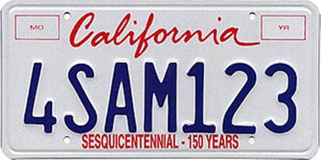
Example: Califoria non-commercial, non-vanity plates have the following generic scheme: $$NLLLNNN$$
Good News: Other kinds probability models are generally a lot harder to construct and we don't expect our Math 2 students to do it.
BUT...................
...we do expect them to be able to use them.
Case in Point: Normal Distributions
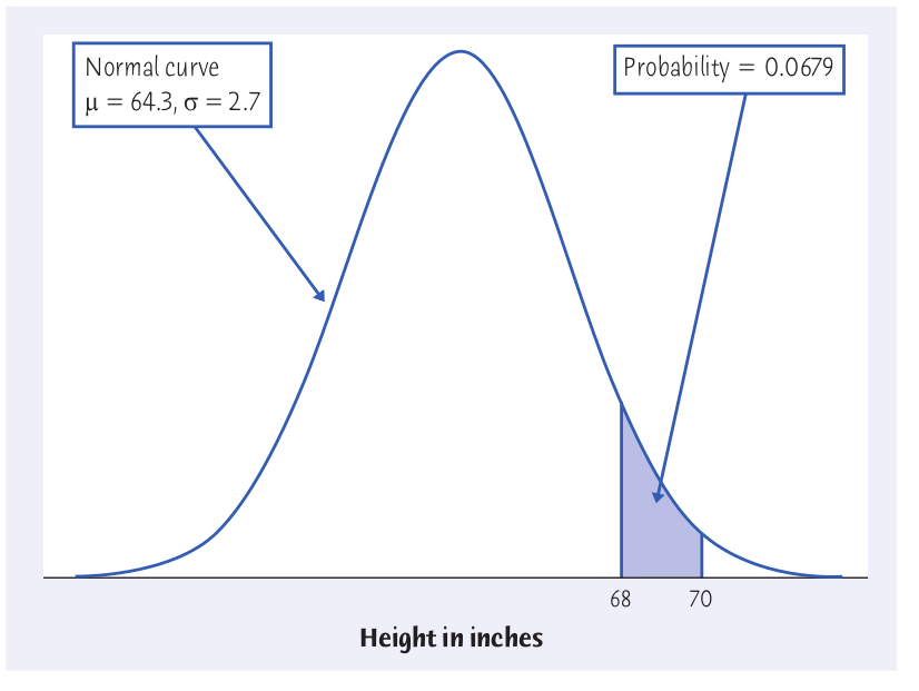
Example: What is the probability that a randomly chosen young womans height $X$ is between 68 and 70 inches tall?
Recall: Young women's heights are distributed normally according to $N(64.3, 2.7)$
We already know how to calculate $P(68 \leq X \leq 70)$.
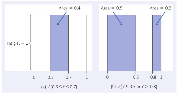
Another Example: Uniform Distributions.
Another Example: Uniform Distributions.
The following is a histogram of computer generated uniform random numbers. The bin width is 0.1.
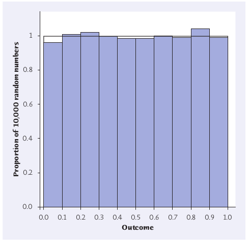
Let's let our computer generate a list of uniform random numbers and paste them into our website stats suite.
How many uniform random numbers: