Polls: When we want to get a sense of how a population feels about an issue, or what candidate they will vote for, we take a poll.
Essentially we want to estimate the percentage, or proportion, of people who will answer in a particular way.
More Generally: when we want to estimate the proportion of observations which fall into a certain category, we use inference for a population proportion.
Other Examples: Estimate the percentage (i.e., proportion) of...
- people who will vote for for a candidate in an upcoming election
- items in a shipment which are defective
- green M&Ms in a typical pack
- people who smoke
- dead trees killed by drought
- things which fall into some category
Estimating Proportions
Draw an SRS of size $n$ from a large population that contains proportion $p$ of successes. Let $\hat{p}$ be the sample proportion of successes, $$\hat{p}=\frac{\mbox{number of successes}}{\mbox{sample size}}$$ Question: what is the sampling distribution of $\hat{p}$?
Answer
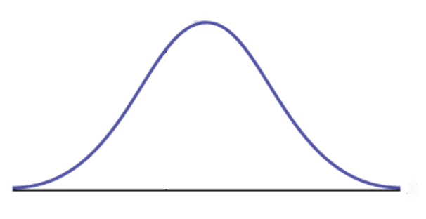
As the sample size increases, the sampling distribution of $\hat{p}$ becomes approximately Normal.
In particular, for large $n$, the sampling distribution of $\hat{p}$ gets closer to $$N\left(p,\sqrt{\frac{p(1-p)}{n}}\right)$$
How to Estimate $p$
Awesome!
So we can just calculate the interval $\displaystyle \hat{p} \pm z^* \sqrt{\frac{p(1-p)}{n}}$...
...right?
An Approximate Confidence Interval
Draw an SRS of size $n$ from a large population that contains an unknown proportion $p$ of successes. An approximate level $C$ confidence interval for $p$ is $$\hat{p} \pm z^* \sqrt{\frac{\hat{p}(1-\hat{p})}{n}}$$ Guideline: Use this interval only when the numbers of successes AND failures in the sample are BOTH $15$ or more.
An Approximate Confidence Interval: Interval Notation
Draw an SRS of size $n$ from a large population that contains an unknown proportion $p$ of successes. An approximate level $C$ confidence interval for $p$ is $$ \left( \hat{p}-z^* \sqrt{\frac{\hat{p}(1-\hat{p})}{n}},\hat{p}+z^* \sqrt{\frac{\hat{p}(1-\hat{p})}{n}} \right)$$ Guideline: Use this interval only when the numbers of successes AND failures in the sample are BOTH $15$ or more.
Example:
$40\%$ of the dots below are pink, and $60\%$ are blue.
Let's pretend we don't know this and
collect a random sample of
dots to estimate the proportion of pink dots with the $95\%$ confidence interval
$\displaystyle \color{red}{\left( \hat{p}-1.96 \sqrt{\frac{\hat{p}(1-\hat{p})}{n}},\hat{p}+1.96 \sqrt{\frac{\hat{p}(1-\hat{p})}{n}} \right)}.$
Example: From a telephone survey of $229$ Americans in the Summer of $1994,$ when asked the question:
"Do you wish Dennis Hopper would go back on drugs?"

$35$ people in the sample answered "yes."
Calculate an approximate $95\%$ confidence interval for the true proportion of Americans who would have answered "yes" to this question.
From the above, we have $k=35$ successes out of $n=229$ observations. This means that there are $194$ failures.
Since the number of successes and failures are BOTH $15$ or more, we may use the large-sample $z$-interval.
We have $\displaystyle \hat{p}=\frac{k}{n}=\frac{35}{229}=0.152$ (to $3$ decimal places).
For $95\%$ confidence, we use $z^{*}=1.960.$ Then $$ \begin{array}{ll} &\displaystyle \left( \hat{p}-z^* \sqrt{\frac{\hat{p}(1-\hat{p})}{n}},\hat{p}+z^* \sqrt{\frac{\hat{p}(1-\hat{p})}{n}} \right)\\ =&\displaystyle \left( 0.152-1.960 \sqrt{\frac{0.152 \cdot 0.848}{229}},0.152+1.960 \sqrt{\frac{0.152 \cdot 0.848}{229}} \right)\\ =&(0.105,0.199)\\ =&(10.5\%,19.9\%)\\ \end{array} $$
Problems
One big problem with these techniques is that they give accurate results only when the sample size is large.
Another problem is with small sample sizes, the counts of successes and failures may be too small, rendering the use of these techniques untrustworthy.
Question: Is there any way to fix this?
The "Plus Four" Confidence Interval.
Suppose you take a sample of size $n$ with $k$ successes. Instead of computing $\displaystyle \hat{p}=\frac{k}{n}$, compute the "plus four" estimate $\displaystyle \tilde{p}=\frac{k+2}{n+4}.$
For smaller sample sizes, the confidence interval $\displaystyle \tilde{p} \pm z^* \sqrt{\frac{\tilde{p}(1-\tilde{p})}{n+4}}$ is usually more accurate.
Guideline: Use this interval when the confidence level is at least $90\%$ and the sample size $n$ is at least $10,$ with any counts of successes and failures.
Example: $40\%$ of the dots below are pink, and $60\%$ are blue. Let's pretend we don't know this and collect a random sample of dots to estimate the proportion of pink dots with the $95\%$ confidence interval $\displaystyle \color{red}{\left( \tilde{p}-1.96 \sqrt{\frac{\tilde{p}(1-\tilde{p})}{n+4}},\tilde{p}+1.96 \sqrt{\frac{\tilde{p}(1-\tilde{p})}{n+4}} \right)}.$
Example: Euro bank notes frequently have detectable traces of cocaine on them.

Suppose researchers collect a sample of $20$ twenty-euro notes and $17$ contained traces of cocaine.
Construct a $95\%$ confidence interval for the proportion $p$ of twenty-euro notes which contain traces of cocaine.
From the above, we have $k=17$ successes out of $n=20$ observations. That means we have $3$ failures.
This means that the guidelines for the large-sample $z$-interval are not met since we require at least $15$ successes AND failures. We shall then use the "plus-four" confidence interval. We shall calculate $\tilde{p}$ instead of $\hat{p}.$
Then $\displaystyle \tilde{p}=\frac{k+2}{n+4}=\frac{17+2}{20+4}=\frac{19}{24}=0.792$ (to $3$ decimal places).
For $95\%$ confidence, we use $z^{*}=1.960.$ Then $$ \begin{array}{ll} &\displaystyle \left( \tilde{p}-z^* \sqrt{\frac{\tilde{p}(1-\tilde{p})}{n+4}},\tilde{p}+z^* \sqrt{\frac{\tilde{p}(1-\tilde{p})}{n+4}} \right)\\ =&\displaystyle \left( 0.792-1.960 \sqrt{\frac{0.792 \cdot 0.208}{24}},0.792+1.960 \sqrt{\frac{0.792 \cdot 0.208}{24}} \right)\\ =&(0.630,0.954)\\ =&(63.0\%,95.4\%)\\ \end{array} $$
Planning a Study: Choosing your sample size.
The margin of error of our large sample confidence interval is $$m=z^*\sqrt{\frac{p(1-p)}{n}}$$ Performing some algebraic shenanigans we get the following nice result...
Planning a Study: Choosing your sample size.
The level $C$ confidence interval for a population proportion $p$ will have margin of error approximately equal to a specified value $m$ when the sample size is $$n=\left(\frac{z^*}{m}\right)^2p^*(1-p^*)$$ where $p^*$ is a guessed value for the sample proportion. The margin of error will always be less than or equal to $m$ if you take the guess $p^*$ to be $0.5.$
Example
The inhabitants of Martiniville, U.S.A. are casting their vote for mayor. On the ballot this election are:
- Sleazy P. Martini (incumbent)
- Stubbs the Cat
Moreover, they all have telephones, they don't lie, and they love to chat on the phone with polsters.
The Situation: We want to estimate the true proportion of Martiniville residents who intend to vote for Stubbs the Cat as mayor within a margin of error of $\pm 3\%$ with $95\%$ confidence. How many people do we need to call?
Another way to ask this is: in repeated samples, how many people would we need to call if we want to get within $3\%$ of the true proportion $95\%$ of the time?
Since we want our margin of error to be $\pm 3\%,$ we take $m=0.03.$
Since our confidence level is $95\%,$ we also have that $z^{*}=1.960.$
We have no idea what $p$ could possibly be, so our guess $p^{*}$ will be $0.5.$ Then, from the formula above we have $$ \begin{array}{ll} n=& \displaystyle \left(\frac{z^*}{m}\right)^2 p^*(1-p^*)\\ =& \displaystyle \left(\frac{1.960}{0.03}\right)^2 (0.5)(0.5)\\ =&1067.\bar{1}\\ \approx & 1068\\ \end{array} $$ Note that we round up so that our margin of error is AT MOST $\pm 3\%.$ Rounding down would mean our margin of error could be larger than $\pm 3\%.$
We have no idea what $p$ could possibly be, so our guess $p^{*}$ will be $0.5.$ Then, from the formula above we have $$ \begin{array}{ll} n=& \displaystyle \left(\frac{z^*}{m}\right)^2 p^*(1-p^*)\\ =& \displaystyle \left(\frac{1.960}{0.03}\right)^2 (0.5)(0.5)\\ =&1067.\bar{1}\\ \approx & 1068\\ \end{array} $$ Note that we round up so that our margin of error is AT MOST $\pm 3\%.$ Rounding down would mean our margin of error could be larger than $\pm 3\%.$
Let's call a sample of residents in Martiniville to estimate the proportion of people who intend to vote for Stubbs the Cat.
Estimate $\hat{p}$: Margin of Error:
Confidence Interval:
Plus Four Confidence Interval:
Calling the Election: Who do you think is going to win?