Systems of ODEs

Systems of ODEs

Systems of ODEs are everywhere in applied mathematics.

Today we will give a crash course in this topic which we could spend a lot more time on.

We shall begin with a motivating example.

Two Interconnected Tanks

Consider two tanks of salt brine that feed into one another.

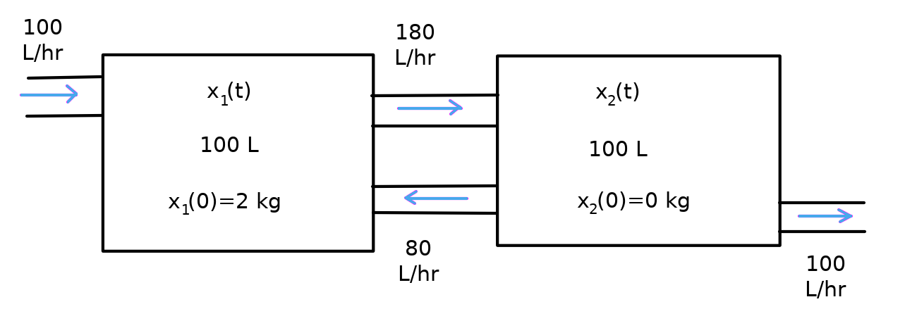
Two Interconnected Tanks

Suppose that two tanks contain $100$ liters of a salt solution with the first tank containing $2$ kilograms of salt and the second containing $0$ kilograms of salt. Beginning as $t=0,$ fresh water begins entering the first tank, and the solution from one tank is being pumped into the other at the rates indicated in the figure below.

Find a system of ODEs which models the amount of salt in each tank at time $t.$

Assume perfect, instantaneous mixing.

Let $x_1$ be the amount of salt in the first tank and let $x_2$ be the amount of salt in the second tank.

For both quantities, we know that $$ x_1'=\mbox{Rate In from Tank 2}-\mbox{Rate Salt Leaves Tank 1} $$ and $$ x_2'=\mbox{Rate In from Tank 1}-\mbox{Rate Salt Leaves Tank 2} $$ Recall that $$ \mbox{Rate In/Out}=\color{magenta}{\mbox{Rate Volume Enters/Exits}}\cdot\color{blue}{\mbox{Salt Concentration}} $$ So, the above equations become $$ x_1'=\underbrace{\color{magenta}{80}\cdot\color{blue}{\frac{x_2}{100}}}_{amount \,\,salt\\entering \,\, from\\tank\,\,2}-\underbrace{\color{magenta}{180}\cdot\color{blue}{\frac{x_1}{100}}}_{amount \,\,salt\\exiting \,\, from\\tank\,\,1} $$ and $$ x_2'=\underbrace{\color{magenta}{180}\cdot\color{blue}{\frac{x_1}{100}}}_{amount \,\,salt\\entering \,\, from\\tank\,\,1}-\underbrace{\color{magenta}{80}\cdot\color{blue}{\frac{x_2}{100}}-\color{magenta}{100}\cdot\color{blue}{\frac{x_2}{100}}}_{amount \,\,salt\\exiting \,\, from\\tank\,\,2} $$ Our system is then $$ x_1'=0.8x_2-1.8 x_1\\ x_2'=1.8x_1-1.8x_2\\ $$ with initial conditions $x_1(0)=2$ and $x_2(0)=0.$

Example

Solve the system $$ x_1'=0.8x_2-1.8 x_1\\ x_2'=1.8x_1-1.8x_2\\ $$ with initial conditions $x_1(0)=2$ and $x_2(0)=0$ using the method of substitution.

Using the first equation, we may rewrite $x_2$ entirely in terms of $x_1.$ $$ x_2=\frac{x_1'+1.8x_1}{0.8} $$ Then, substituting this into the second equation, $$ \begin{array}{lll} &\displaystyle x_2'=1.8x_1-1.8x_2&\mbox{}\\ \implies &\displaystyle \left(\frac{x_1'+1.8x_1}{0.8}\right)'=1.8x_1-1.8\cdot \frac{x_1'+1.8x_1}{0.8}&\mbox{}\\ \implies &\displaystyle \frac{x_1''+1.8x_1'}{0.8}=1.8x_1-1.8\frac{x_1'+1.8x_1}{0.8}&\mbox{}\\ \implies &\displaystyle x_1''+1.8x_1'=0.8\cdot 1.8x_1-1.8(x_1'+1.8x_1)&\mbox{}\\ \implies &\displaystyle x_1''+1.8x_1'=1.44x_1-1.8x_1'-3.24x_1&\mbox{}\\ \implies &\displaystyle x_1''+1.8x_1'=-1.8x_1'-1.8x_1&\mbox{}\\ \implies &\displaystyle x_1''+3.6x_1'+1.8x_1=0&\mbox{}\\ \end{array} $$ This is a second-order linear equation we can solve!

The characteristic equation is $$ r^2+3.6r+1.8=0 $$ so that $$ r=-0.6\,\,\,\,\mbox{or}\,\,\,\,r=-3 $$ That is, $$ x_1=C_1e^{-0.6t}+C_2e^{-3t} $$ From our original substitution, $$ \begin{array}{lll} \displaystyle x_2&\displaystyle=\frac{x_1'+1.8x_1}{0.8} &\mbox{}\\ \displaystyle &\displaystyle=\frac{(C_1e^{-0.6t}+C_2e^{-3t})'+1.8(C_1e^{-0.6t}+C_2e^{-3t})}{0.8} &\mbox{}\\ \displaystyle &\displaystyle=\frac{-0.6C_1e^{-0.6t}-3C_2e^{-3t}+1.8C_1e^{-0.6t}+1.8C_2e^{-3t}}{0.8} &\mbox{}\\ \displaystyle &\displaystyle=\frac{1.2C_1e^{-0.6t}-1.2C_2e^{-3t}}{0.8} &\mbox{}\\ \displaystyle &\displaystyle=1.5C_1e^{-0.6t}-1.5C_2e^{-3t} &\mbox{}\\ \end{array} $$ And the system is solved in general!

Imposing the initial conditions, $$ \begin{array}{lll} &\displaystyle x_1(0)=2\,\,\,\,\mbox{and}\,\,\,\, x_2(0)=0&\mbox{}\\ \implies &\displaystyle C_1e^{-0.6\cdot 0}+C_2e^{-3\cdot 0}=2\,\,\,\,\mbox{and}\,\,\,\, 1.5C_1e^{-0.6\cdot 0}-1.5C_2e^{-3\cdot 0}=0&\mbox{}\\ \implies &\displaystyle C_1+C_2=2\,\,\,\,\mbox{and}\,\,\,\, 1.5C_1-1.5C_2=0&\mbox{}\\ \end{array} $$ By inspection, $C_1=1$ and $C_2=1.$

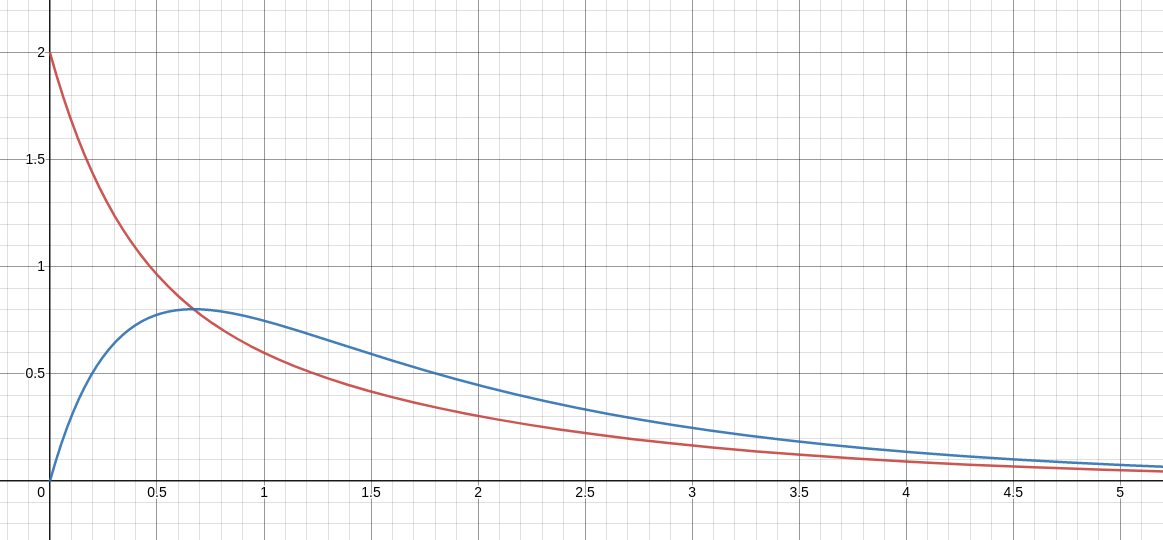
The solution for this situation is then $$ \begin{array}{l} x_1(t)=e^{-0.6t}+e^{-3t}\\ x_2(t)=1.5e^{-0.6t}-1.5e^{-3t}\\ \end{array} $$ A graph of our pair of solutions is shown below.

The Method of Substitution

Step $1:$ Solve for one variable in terms of the other in one equation.

Step $2:$ Substitute the resulting equation from above into the other equation. The result should be a second-order linear equation in a single variable.

Step $3:$ Solve the second-order equation.

Step $4:$ Use the equation obtained in Step $1$ to solve for the other variable.

Step $5:$ Satisfy initial conditions if necessary.

If the system contains more than $2$ variables, use back substitution to get a single higher-order equation in a single variable.

Techniques for Solving Systems

Most systems we solve are linear.

If the system is nonlinear, we either linearize the system or use numerical methods.

This is to say that solving systems of ODEs begins with solving linear systems.

The techniques we shall presently illustrate are:

1) The Method of Substitution

2) Laplace Transform Methods

3) Matrix Methods.

4) Numerical Methods (i.e., Runge-Kutta for Systems)

Solving Systems Using the Laplace Transform.

Suppose we have a linear, constant coefficient system of ODEs $$ x_1'=a_{1,1}x_1+a_{1,2}x_{2}+\cdots+a_{1,n-1}x_{n-1}+a_{1,n}x_n\\ x_2'=a_{2,1}x_1+a_{2,2}x_{2}+\cdots+a_{2,n-1}x_{n-1}+a_{2,n}x_n\\ \vdots\\ %x_{n-1}'=a_{n-1,1}x_1+a_{n-1,2}x_{2}+\cdots+a_{n-1,n-1}x_{n-1}+a_{n-1,n}x_n\\ x_n'=a_{n,1}x_1+a_{n,2}x_{2}+\cdots+a_{n,n-1}x_{n-1}+a_{n,n}x_n $$ To solve an IVP involving this system, take the Laplace transform of each equation, $$ sX_1-x_1(0)=a_{1,1}X_1+a_{1,2}X_{2}+\cdots+a_{1,n-1}X_{n-1}+a_{1,n}X_n\\ sX_2-x_2(0)=a_{2,1}X_1+a_{2,2}X_{2}+\cdots+a_{2,n-1}X_{n-1}+a_{2,n}X_n\\ \vdots\\ sX_n-x_n(0)=a_{n,1}X_1+a_{n,2}X_{2}+\cdots+a_{n,n-1}X_{n-1}+a_{n,n}X_n $$ and solve for each $X_j$ algebraically using familiar methods.

Then take the inverse transform of both sides to solve for each $x_j.$

Example

Solve the system $$ x_1'=0.8x_2-1.8 x_1\\ x_2'=1.8x_1-1.8x_2\\ $$ with initial conditions $x_1(0)=2,$ $x_2(0)=0$ using the Laplace transform.

Taking the Laplace transform of each equation we have $$ sX_1-x_1(0)=0.8X_2-1.8 X_1\\ sX_2-x_2(0)=1.8X_1-1.8X_2 $$ which imposing the initial conditions becomes $$ \begin{array}{l} sX_1-2=0.8X_2-1.8 X_1\\ sX_2=1.8X_1-1.8X_2\\ \end{array} $$ Rearranging, $$ \begin{array}{r} (s+1.8)X_1-0.8X_2=2\\ -1.8X_1+(s+1.8)X_2=0\\ \end{array} $$ Using Cramer's Rule (or elimination, or any other method for solving algebraic systems), $$ X_1=\frac{\left|\begin{array}{cc}2&-0.8\\0&s+1.8\\ \end{array}\right|}{\left|\begin{array}{cc} s+1.8&-0.8\\-1.8&s+1.8\\ \end{array}\right|}, \,\,\,\, X_2=\frac{\left|\begin{array}{cc} s+1.8&2\\-1.8&0\\ \end{array}\right|}{\left|\begin{array}{cc} s+1.8&-0.8\\-1.8&s+1.8\\ \end{array}\right|} $$ That is, $$ \begin{array}{lll} \displaystyle X_1&\displaystyle=\frac{2(s+1.8)-(-0.8)(0)}{(s+1.8)^2-(-0.8)(-1.8)} &\mbox{}\\ \displaystyle &\displaystyle=\frac{2(s+1.8)}{(s+1.8)^2-1.44} &\mbox{}\\ \displaystyle &\displaystyle=\frac{2(s+1.8)}{(s+1.8)^2-1.2^2} &\mbox{}\\ \end{array} $$ Taking the inverse transform, $$ \begin{array}{lll} \displaystyle x_1&\displaystyle=\mathscr{L}^{-1}\left\{\frac{2(s+1.8)}{(s+1.8)^2-1.2^2}\right\} &\mbox{}\\ \displaystyle &\displaystyle=2\mathscr{L}^{-1}\left\{\frac{s+1.8}{(s+1.8)^2-1.2^2}\right\}&\mbox{}\\ \displaystyle &\displaystyle=2e^{-1.8t}\cosh(1.2t) &\mbox{}\\ \displaystyle &\displaystyle=2e^{-1.8t}\cdot\frac{e^{1.2t}+e^{-1.2t}}{2} &\mbox{}\\ \displaystyle &\displaystyle=e^{-0.6t}+e^{-3t} &\mbox{}\\ \end{array} $$ Also, $$ \begin{array}{lll} \displaystyle X_2&\displaystyle=\frac{(s+1.8)(0)-(2)(-1.8)}{(s+1.8)^2-(-0.8)(-1.8)} &\mbox{}\\ \displaystyle &\displaystyle=\frac{2(1.8)}{(s+1.8)^2-1.44} &\mbox{}\\ \displaystyle &\displaystyle=\frac{2(1.8)}{(s+1.8)^2-1.2^2} &\mbox{}\\ \displaystyle &\displaystyle=\frac{2(1.8)}{\color{magenta}{1.2}}\frac{\color{magenta}{1.2}}{(s+1.8)^2-1.2^2} &\mbox{}\\ \displaystyle &\displaystyle=3\frac{1.2}{(s+1.8)^2-1.2^2} &\mbox{}\\ \end{array} $$ so that $$ \begin{array}{lll} \displaystyle x_2&\displaystyle=3\mathscr{L}^{-1}\left\{\frac{1.2}{(s+1.8)^2-1.2^2}\right\} &\mbox{}\\ \displaystyle &\displaystyle=3e^{-1.8t}\sinh(1.2t) &\mbox{}\\ \displaystyle &\displaystyle=3e^{-1.8t}\cdot\frac{e^{1.2t}-e^{-1.2t}}{2} &\mbox{}\\ \displaystyle &\displaystyle=1.5e^{-0.6t}-1.5e^{-3t} &\mbox{}\\ \end{array} $$

Matrix Methods for Solving Homogeneous Constant-Coefficient Systems

If the constant matrix $A$ has $n$ linearly independent eigenvalues $\lambda_1,\cdots \lambda_n,$ and eigenvectors ${\bf v}_1,\cdots {\bf v}_n,$ then $$ {\bf x}(t)=C_1{\bf v}_1e^{\lambda_1 t}+C_2{\bf v}_2e^{\lambda_2 t}+\cdots+C_n{\bf v}_ne^{\lambda_n t} $$ is the general solution to the system of ODEs expressed in matrix form. $${\bf x}'=A{\bf x}$$

Example

Solve the system $$ x_1'=0.8x_2-1.8 x_1\\ x_2'=1.8x_1-1.8x_2\\ $$ with initial conditions $x_1(0)=2,$ $x_2(0)=0$ using matrix methods.

We first write the system as $$ x_1'=-1.8 x_1+0.8x_2\\ x_2'=1.8x_1-1.8x_2\\ $$ so that the IVP in matrix form is $$ {\bf x}'=\left[\begin{array}{c}x_1'\\x_2'\end{array}\right]=\left[\begin{array}{cc}-1.8&0.8\\1.8&-1.8\end{array}\right]\left[\begin{array}{c}x_1\\x_2\end{array}\right]=A{\bf x}, \,\,\,\, {\bf x}(0)=\left[\begin{array}{c}2\\0\end{array}\right] $$ The eigenvalues of the coefficient matrix are $$ \lambda_1=-0.6 \,\,\,\,\mbox{and}\,\,\,\, \lambda_2=-3 $$ with corresponding, linearly independent, eigenvectors $$ {\bf v}_1=\left[\begin{array}{c}1\\1.5\end{array}\right] \,\,\,\,\mbox{and}\,\,\,\, {\bf v}_2=\left[\begin{array}{c}1\\-1.5\end{array}\right] $$ The general solution to the system is then $$ \begin{array}{lll} \displaystyle{\bf x}(t) &\displaystyle=\left[\begin{array}{c}x_1\\x_2\end{array}\right] &\mbox{}\\ \displaystyle &\displaystyle=C_1{\bf v}_1e^{\lambda_1}+C_2{\bf v}_2e^{\lambda_2} &\mbox{}\\ \displaystyle &\displaystyle=C_1\left[\begin{array}{c}1\\1.5\end{array}\right]e^{-0.6t}+C_2\left[\begin{array}{c}1\\-1.5\end{array}\right]e^{-3t} &\mbox{}\\ \displaystyle &\displaystyle=\left[\begin{array}{c}C_1e^{-0.6t}\\1.5C_1e^{-0.6t}\end{array}\right]+\left[\begin{array}{c}C_2e^{-3t}\\-1.5C_2e^{-3t}\end{array}\right] &\mbox{}\\ \displaystyle &\displaystyle=\left[\begin{array}{c}C_1e^{-0.6t}+C_2e^{-3t}\\1.5C_1e^{-0.6t}-1.5C_2e^{-3t}\end{array}\right] &\mbox{}\\ \end{array} $$ Satisfying initial conditions, $$ \begin{array}{lll} &\displaystyle {\bf x}(0)=\left[\begin{array}{c}2\\0\end{array}\right] &\mbox{}\\ \implies &\displaystyle \left[\begin{array}{c}C_1e^{-0.6\cdot 0}+C_2e^{-3\cdot 0}\\1.5C_1e^{-0.6\cdot 0}-1.5C_2e^{-3\cdot 0}\end{array}\right]=\left[\begin{array}{c}2\\0\end{array}\right] &\mbox{}\\ \implies &\displaystyle \left[\begin{array}{c}C_1+C_2\\1.5C_1-1.5C_2\end{array}\right]=\left[\begin{array}{c}2\\0\end{array}\right] &\mbox{}\\ \implies &\displaystyle \left[\begin{array}{cc}1&1\\1.5&-1.5\end{array}\right] \left[\begin{array}{c}C_1\\C_2\end{array}\right]=\left[\begin{array}{c}2\\0\end{array}\right] &\mbox{}\\ \implies &\displaystyle \left[\begin{array}{c}C_1\\C_2\end{array}\right]=\left[\begin{array}{cc}1&1\\1.5&-1.5\end{array}\right]^{-1}\left[\begin{array}{c}2\\0\end{array}\right] &\mbox{}\\ \implies &\displaystyle \left[\begin{array}{c}C_1\\C_2\end{array}\right]=\left[\begin{array}{cc}\frac{1}{2}&\frac{1}{3}\\\frac{1}{2}&-\frac{1}{3}\end{array}\right]\left[\begin{array}{c}2\\0\end{array}\right] &\mbox{}\\ \implies &\displaystyle \left[\begin{array}{c}C_1\\C_2\end{array}\right]=\left[\begin{array}{c}1\\1\end{array}\right] &\mbox{}\\ \end{array} $$ The solution to the IVP is then $$ \begin{array}{lll} \displaystyle{\bf x}(t) &\displaystyle=\left[\begin{array}{c}e^{-0.6t}+e^{-3t}\\1.5e^{-0.6t}-1.5e^{-3t}\end{array}\right] &\mbox{}\\ \end{array} $$

More General Systems of ODEs

We have seen an example of a first-order, linear, homogeneous, constant-coefficient system of ODEs.

In general, any first-order system in two variables can be written in the form $$ x_1'=f_1(x_1,x_2,t)\\ x_2'=f_2(x_1,x_2,t) $$ where $f_1$ and $f_2$ are functions of three variables.

Example $$ \begin{array}{l} x_1'=t^2x_1+5x_2+\sin t\\ x_2'=e^t x_1-x_2+\cos t\\ \end{array} $$

Runge-Kutta Methods for First-Order Systems $$ x_1'=f_1(x_1,x_2,t),\,\,\,\,\,x_1(0)=a_1\\ x_2'=f_2(x_1,x_2,t),\,\,\,\,\,x_2(0)=a_2 $$ To approximate the above initial value problem choose a step size $h.$ Then compute $$ \begin{array}{l} t_{n+1}=t_n+h\\ x_{n+1,2}=x_{n+1,1}+\frac{1}{6}(k_{1,1}+2k_{2,1}+2k_{3,1}+k_{4,1})\\ x_{n+1,2}=x_{n+1,2}+\frac{1}{6}(k_{1,2}+2k_{2,2}+2k_{3,2}+k_{4,2})\\ \end{array} $$ where $$ \begin{array}{l} k_{1,1}=hf_1(x_{n,1},x_{n,2},t_n)\\ k_{1,2}=hf_2(x_{n,1},x_{n,2},t_n)\\ k_{2,1}=hf_1\left(x_{n,1}+0.5k_{1,1},x_{n,2}+0.5k_{1,2},t+0.5h\right)\\ k_{2,2}=hf_2\left(x_{n,1}+0.5k_{1,1},x_{n,2}+0.5k_{1,2},t+0.5h\right)\\ k_{3,1}=hf_1\left(x_{n,1}+0.5k_{2,1},x_{n,2}+0.5k_{2,2},t+0.5h\right)\\ k_{3,2}=hf_2\left(x_{n,1}+0.5k_{2,1},x_{n,2}+0.5k_{2,2},t+0.5h\right)\\ k_{4,1}=hf_1(x_{n,1}+k_{3,1},x_{n,2}+k_{3,2},t_n+h)\\ k_{4,2}=hf_2(x_{n,1}+k_{3,1},x_{n,2}+k_{3,2},t_n+h)\\ \end{array} $$

Example

Solve the system $$ x_1'=0.8x_2-1.8 x_1\\ x_2'=1.8x_1-1.8x_2 $$ using Runge-Kutta methods with initial conditions:

$\displaystyle x_1(0)=$, $\displaystyle x_2(0)=$ See exact solution.

	Amount of Salt in Tank 1		Amount of Salt in Tank 2		Phase Plane Trajectory
$x_1$		$x_2$		$x_2$
	$t$		$t$		$x_1$

Coupled Mass-Spring Systems

An example ofa coupled mass spring system is the following pictured below.

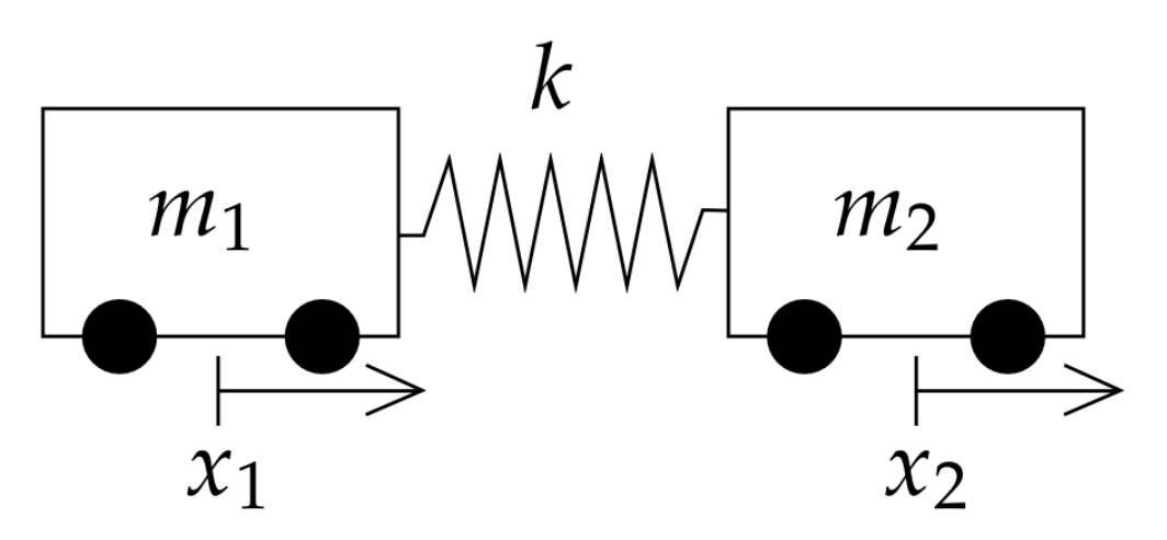
Letting $x_1$ be the displacement of the first mass from its initial rest position, and $x_2$ be the displacement of the second mass from its initial rest position, and assuming our rolling masses experience no friction, the only forces the masses experience is from the attached spring. From Newton's Second Law, $$ m_1x_1''=\mbox{net force on $m_1$}=k(x_2-x_1)\\ m_2x_2''=\mbox{net force on $m_2$}=k(x_1-x_2)\\ $$

Coupled Mass-Spring Systems

Another example of a coupled mass spring system is the following pictured below.

Letting $x_1$ be the displacement of the first mass from its initial rest position, and $x_2$ be the displacement of the second mass from its initial rest position, and assuming our rolling masses experience no friction, the only forces the masses experience is from the attached spring. From Newton's Second Law, $$ \begin{array}{lll} m_1x_1''&=\mbox{net force on $m_1$}&=k_2(x_2-x_1)-k_1x_1\\ m_2x_2''&=\mbox{net force on $m_2$}&=k_2(x_1-x_2)\\ \end{array} $$

Coupled Mass-Spring Systems

Yet another example of a coupled mass spring system is the following pictured below.

Letting $x_1$ be the displacement of the first mass from its initial rest position, $x_2$ be the displacement of the second mass from its initial rest position, and $x_3$ be the displacement of the second mass from its initial rest position. Assuming our rolling masses experience no friction, the only forces the masses experience is from the attached spring. From Newton's Second Law, $$ \begin{array}{lll} m_1x_1''=\mbox{net force on $m_1$}=-k_1x_1+k_2(x_2-x_1)\\ m_2x_2''=\mbox{net force on $m_2$}=-k_2(x_2-x_1)+k_3(x_3-x_2)\\ m_3x_3''=\mbox{net force on $m_3$}=-k_3(x_3-x_2)-k_4x_3\\ \end{array} $$

Example

Suppose, as seen in the figure below, a $m_1=2$ kg rolling mass is attached to a wall with a spring constant of $k_1=4$ newtons per meter. The mass is coupled to another $m_2=1$ kg rolling mass via a spring with spring constant of $k_2=2$ newtons per meter.

Both carts are placed $3$ meters above their equilibrium positions and released.

Find the positions of each mass. That is, solve the second-order system $$ \begin{array}{lll} 2x_1''&=2(x_2-x_1)-4x_1&=-6x_1+2x_2\\ x_2''&=2(x_1-x_2)&=2x_1-2x_2\\ \end{array} $$ with initial conditions $x_1(0)=x_2(0)=3$ and $x_1'(0)=x_2'(0)=0.$

Dividing the first equation by $2,$ we have $$ x_1''=-3x_1+x_2 $$ so that $$ x_2=3x_1+x_1'' $$ Substituting into the second equation, $$ \begin{array}{lll} &\displaystyle x_2''=2x_1-2x_2&\mbox{}\\ \implies &\displaystyle (3x_1+x_1'')''=2x_1-2(3x_1+x_1'')&\mbox{}\\ \implies &\displaystyle 3x_1''+x_1^{(4)}=2x_1-6x_1-2x_1''&\mbox{}\\ \implies &\displaystyle x_1^{(4)}+3x_1''=-4x_1-2x_1''&\mbox{}\\ \implies &\displaystyle x_1^{(4)}+5x_1''+4x_1=0&\mbox{}\\ \end{array} $$ Solving the characteristic equation, $$ \begin{array}{lll} &\displaystyle r^4+5r^2+4=0 &\mbox{}\\ \implies &\displaystyle r^2=\frac{-5\pm\sqrt{5^2-4(1)(4)}}{2(1)}&\mbox{}\\ \implies &\displaystyle r^2=\frac{-5\pm\sqrt{9}}{2}&\mbox{}\\ \implies &\displaystyle r^2=\frac{-5\pm 3}{2}&\mbox{}\\ \implies &\displaystyle r^2=\frac{-2}{2} \,\,\,\,\mbox{or}\,\,\,\, r^2=\frac{-8}{2}&\mbox{}\\ \implies &\displaystyle r^2=-1 \,\,\,\,\mbox{or}\,\,\,\, r^2=-4&\mbox{}\\ \implies &\displaystyle r=\pm i \,\,\,\,\mbox{or}\,\,\,\, r=\pm 2i&\mbox{}\\ \end{array} $$ It follows that $$ x_1=C_1 \cos t+C_2 \sin t+C_3 \cos(2t)+C_4\sin(2t) $$ Then, $$ \begin{array}{lll} \displaystyle x_2&\displaystyle=3x_1+x_1'' &\mbox{}\\ \displaystyle &\displaystyle=3(C_1 \cos t+C_2 \sin t+C_3 \cos(2t)+C_4\sin(2t))+(C_1 \cos t+C_2 \sin t+C_3 \cos(2t)+C_4\sin(2t))'' &\mbox{}\\ \displaystyle &\displaystyle=3C_1 \cos t+3C_2 \sin t+3C_3 \cos(2t)+3C_4\sin(2t))-C_1 \cos t-C_2 \sin t-4C_3 \cos(2t)-4C_4\sin(2t) &\mbox{}\\ \displaystyle &\displaystyle=2C_1 \cos t+2C_2 \sin t-C_3 \cos(2t)-C_4\sin(2t) &\mbox{}\\ \end{array} $$ We now satisfy the initial conditions. $$ \begin{array}{lll} &\displaystyle x_1(0)=3\,\,\,\,\mbox{and}\,\,\,\,x_2(0)=3&\mbox{}\\ \implies &\displaystyle C_1 \cos 0+C_2 \sin 0+C_3 \cos(2\cdot 0)+C_4\sin(2\cdot 0)=3 \,\,\,\,\mbox{and}\,\,\,\,2C_1 \cos 0+2C_2 \sin 0-C_3 \cos(2\cdot 0)-C_4\sin(2\cdot 0)=3&\mbox{}\\ \implies &\displaystyle C_1+C_3 =3 \,\,\,\,\mbox{and}\,\,\,\,2C_1-C_3=3&\mbox{}\\ \end{array} $$ Adding the two resulting equations, we get $3C_1=6$ so that $C_1=2.$ Consequently, $C_3=1.$

Now, since $$x_1'=-C_1 \sin t+C_2 \cos t-2C_3 \sin(2t)+2C_4\cos(2t)$$ and $$x_2'=-2C_1 \sin t+2C_2 \cos t+2C_3 \sin(2t)-2C_4\cos(2t)$$ we have $$ \begin{array}{lll} &\displaystyle x_1'(0)=0\,\,\,\,\mbox{and}\,\,\,\,x_2'(0)=0&\mbox{}\\ \implies &\displaystyle -C_1 \sin 0+C_2 \cos 0-2C_3 \sin(2\cdot 0)+2C_4\cos(2\cdot 0)=0 \,\,\,\,\mbox{and}\,\,\,\,-2C_1 \sin 0+2C_2 \cos 0+2C_3 \sin(2\cdot 0)-2C_4\cos(2\cdot 0)=0&\mbox{}\\ \implies &\displaystyle C_2 +2C_4=0 \,\,\,\,\mbox{and}\,\,\,\,2C_2 -2C_4=0&\mbox{}\\ \end{array} $$ By inspection, $C_2=0$ and $C_4=0$

Our solution is then $$ x_1=2\cos t+\cos(2t)\\ x_2=4\cos t-\cos(2t) $$

Coupled Mass-Spring Animation

$ \begin{array}{ll} 2\color{#cc5652}{x_1}''&=2(\color{#417eba}{x_2}-\color{#cc5652}{x_1})-4\color{#cc5652}{x_1}\\ \color{#417eba}{x_2}''&=2(\color{#cc5652}{x_1}-\color{#417eba}{x_2})\\ \end{array} $

Systems of ODEs in General

We have now seen examples of both first and second-order systems of ODEs.

In general, any second-order system in two variables can be written in the form $$ x_1''=f_1(x_1,x_2,x_1',x_2',t)\\ x_2''=f_2(x_1,x_2,x_1',x_2',t) $$ For reasons which will soon become apparent, we may focus our attention on first-order systems.

Systems of ODEs in General

Any first-order system in $n$ variables can be written in the form $$ x_1'=f_1(x_1,x_2,\cdots, x_n,t)\\ x_2'=f_2(x_1,x_2,\cdots, x_n,t)\\ \vdots\\ x_n'=f_n(x_1,x_2,\cdots, x_n,t)\\ $$

Great News!

In previous examples, we have seen that solving a first-order system of equations can be reduced to solving a single, higher-order ODE.

For example, we saw that solving the system $$ x_1'=0.8x_2-1.8 x_1\\ x_2'=1.8x_1-1.8x_2 $$ was reduced to solving the second-order equation $$ x_1''+3.6x_1'+1.8x_1=0 $$ It turns out that sometimes the opposite is what we need.

That is, it is quite useful being able to turn a single higher-order equation into a system.

We will first state the general procedure.

Turning $n$th-Order Equations into First-Order Systems

To convert the single $n$th-order equation $$ y^{(n)}=f(y,y',y'',\ldots,y^{(n-1)},t) $$ into a first-order system, make the substitutions $$ \begin{array}{rl} x_1&=y\\ x_2&=y'\\ &\vdots\\ x_{n}&=y^{(n-1)}\\ \end{array} $$ Then....

Turning $n$th-Order Equations into First-Order Systems

The equation $$ y^{(n)}=f(y,y',y'',\ldots,y^{(n-1)},t) $$ is equivalent to the system $$ \begin{array}{rl} x_1'&=y'=x_2\\ x_2'&=y''=x_3\\ &\vdots\\ x_n'&=y^{n}=f(x_1,x_2,x_3,\ldots,x_{n-1},t)\\ \end{array} $$

Example

Convert the second-order linear equation $$ y''+t^2y'-e^ty=\cos t $$ into a first-order system of two equations in two dependent variables.

Let $x_1=y$ and $x_2=y'.$

Then $$ \begin{array}{l} x_1'=y'=x_2\\ x_2'=y''=-t^2y'+e^ty+\cos t=-t^2x_2+e^t x_1+\cos t \end{array} $$ Or, in a more cleaned-up form, $$ \begin{array}{llrl} x_1'&=&x_2&\\ x_2'&=e^t x_1&-t^2x_2&+\cos t \end{array} $$

Turning a Second-Order System into a First-Order System

We've already seen that any $n$th-order equation can be converted into an equivalent first-order system.

It turns out that second-order systems can also be restated as first-order systems too.

In fact, any system or equation can be formulated into an equivalent first-order system.

And since numerical methods like Runge-Kutta generally work great with first-order systems, the world is our oyster!

Example

Convert the second-order system $$ m_1x_1''=k(x_2-x_1)\\ m_2x_2''=k(x_1-x_2)\\ $$ into a first-order system.

We will introduce the substitutions $$ u_1=x_1\\ u_2=x_1'\\ u_3=x_2\\ u_4=x_2' $$ Then, $$ \begin{array}{l} u_1'=x_1'=u_2\\ u_2'=x_1''=\frac{k}{m_1}(x_2-x_1)=\frac{k}{m_1}(u_3-u_1)\\ u_3'=x_2'=u_4\\ u_4'=x_2''=\frac{k}{m_1}(x_2-x_1)=\frac{k}{m_1}(u_1-u_3) \end{array} $$ Or, $$ \begin{array}{ll} u_1'&=&&u_2&&\\ u_2'&=&-\frac{k}{m_1}u_1&&+\frac{k}{m_1}u_3&\\ u_3'&=&&&&u_4\\ u_4'&=&\frac{k}{m_1}u_1&&-\frac{k}{m_1}u_3&\\ \end{array} $$

Bonus Example

Taking $\displaystyle \frac{g}{L}=1,$ convert the nonlinear pendulum equation $$ \displaystyle \frac{d^2\theta}{dt^2}+\frac{g}{L}\sin \theta=0 $$ into a first-order system.

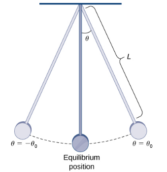
The equation with the given information is $$ \theta''+\sin \theta=0 $$ To convert to a first-order system we let $x_1=\theta$ and $x_2=\theta'.$

Then $$ x_1'=\theta'=x_2\\ $$ and $$ x_2'=\theta''=-\sin \theta=-\sin x_1 $$ Our cleaned-up system is then $$ \begin{array}{ll} x_1'&=&&x_2\\ x_2'&=&-\sin x_1&\\ \end{array} $$

Bonus Application of Runge-Kutta to Pendulum Problem!

Solve the system $$ \begin{array}{ll} x_1'&=&&x_2\\ x_2'&=&-\sin x_1 &\\ \end{array} $$ using Runge-Kutta methods with initial conditions:

$\displaystyle x_1(0)=$, $\displaystyle x_2(0)=$ See linearized solution.

					Phase Plane Trajectory
$\theta\\=\\x_1$		$\theta'\\=\\x_2$		$x_2$
	$t$		$t$		$x_1$

Autonomous Systems

A first-order system $n$ variables is called autonomous if the derivatives of each dependent variable can be expressed solely in terms of the other dependent variables.

That is, if it can be written in the form $$ x_1'=f_1(x_1,x_2,\cdots, x_n)\\ x_2'=f_2(x_1,x_2,\cdots, x_n)\\ \vdots\\ x_n'=f_n(x_1,x_2,\cdots, x_n)\\ $$ Each derivative $x_j'$ doesn't depend on $t.$

Autonomous Systems

The advantage to autonomous systems is that we can visualize solutions with phase portraits (a multidimensional version of a phase line).

$ \begin{array}{l} \mbox{System}\\ x'=y\\ y'=-\sin(x)\\ \\ \mbox{Direction Field}\\ \langle y,-\sin(x)\rangle\\ \\ \mbox{Slope Field}\\ \displaystyle \frac{dy}{dx}=\frac{-\sin(x)}{y} \end{array} $

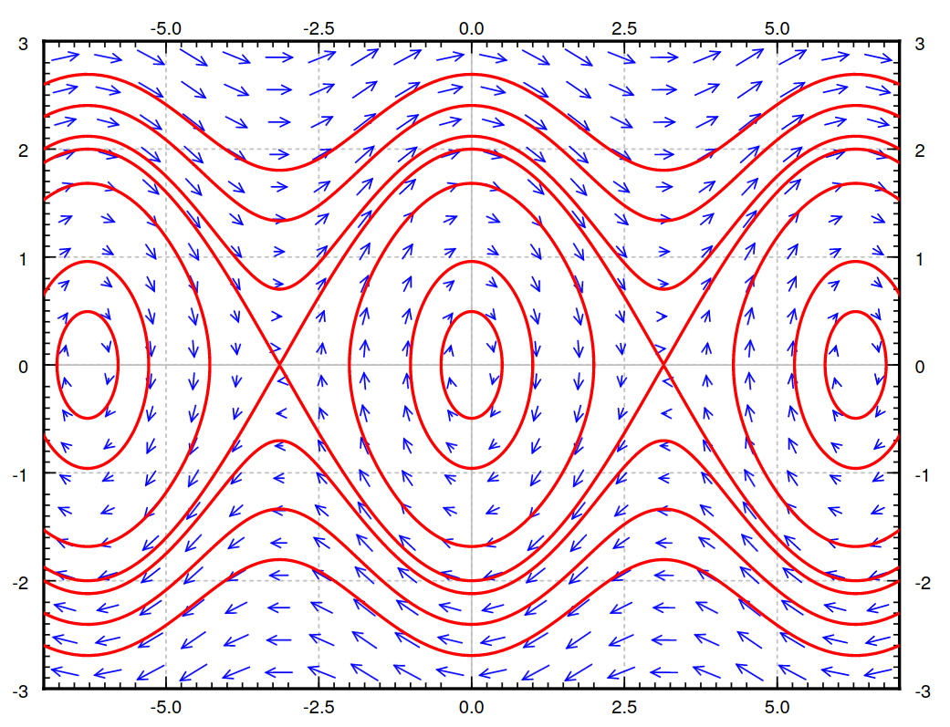
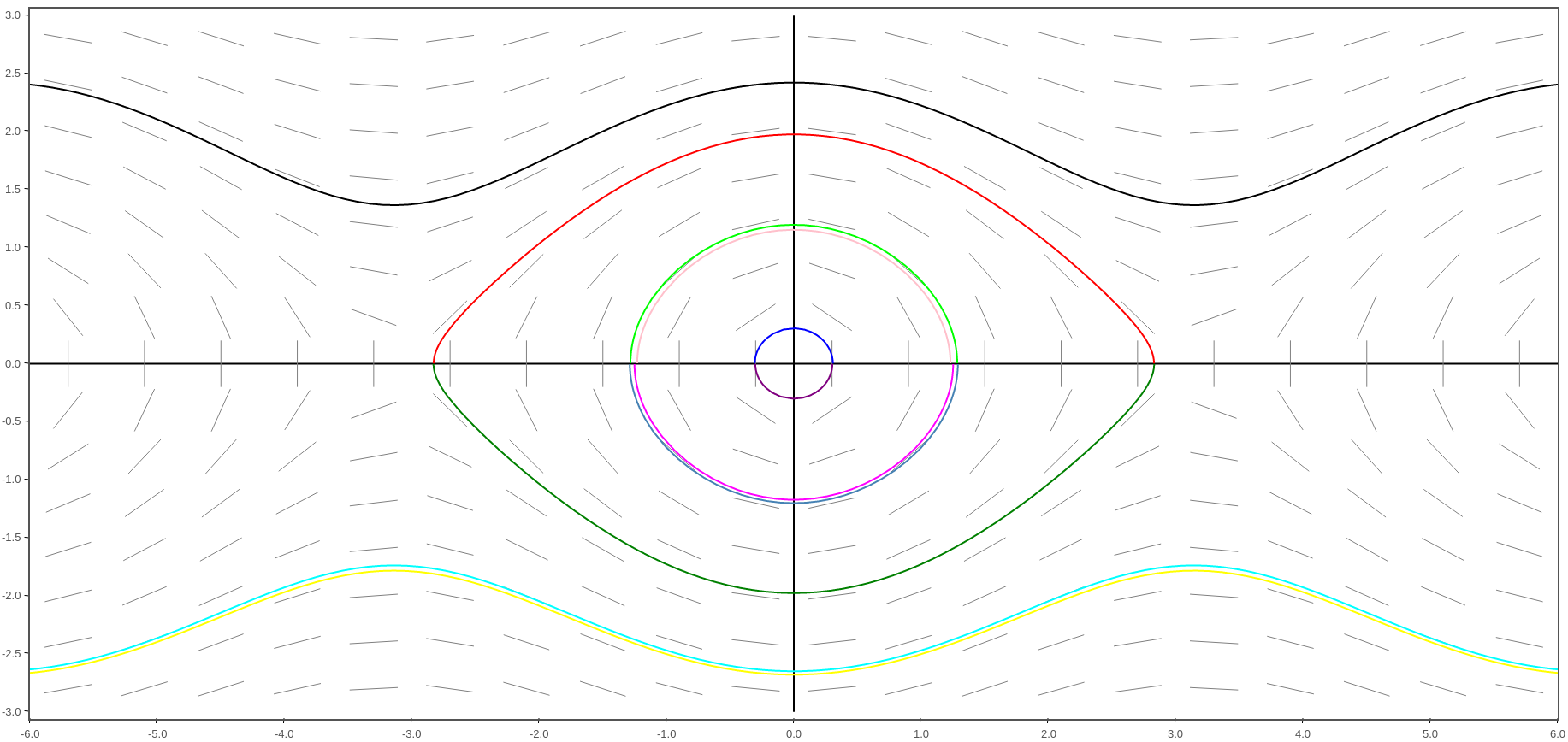
This type of analysis we will not pursue here, but do know that it's the beginning of understanding nonlinear systems.

Another nice thing about autonomous systems is that finding equilibrium points is an algebraic problem.

Other Applications of Systems: Compartmental Models

Example: Levels of pollution in the Great Lakes.

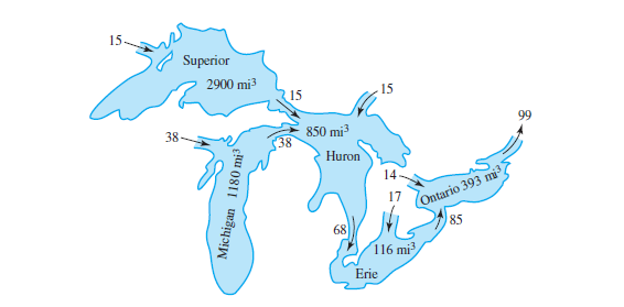
Our tank problem nicely sets the stage for solving problems like these.

Other Applications of Systems: Compartmental Models

Example: The (Nonlinear) SIR Model $$ \begin{array}{l} \displaystyle S'=-\frac{\beta IS}{N},\,\,\,\,\,\,\,\, \\ \displaystyle I'=\frac{\beta IS}{N}-\gamma I,\,\,\,\,\,\,\,\, \\ \displaystyle R'=\gamma I \end{array} $$

Other Applications of Systems: Population Dynamics

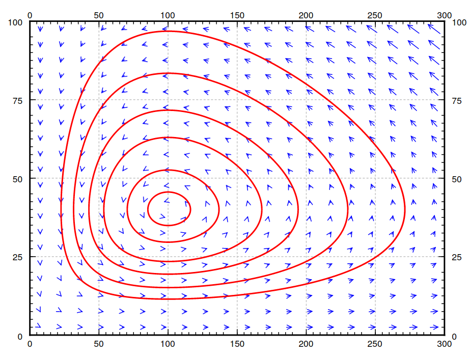
The nonlinear system $$ \begin{array}{l} x_1'=(A-B x_2)x_1\\ x_2'=(Cx_1-D)x_2\\ \end{array} $$ is the well-known Lotka-Volterra model for predator/prey interactions.

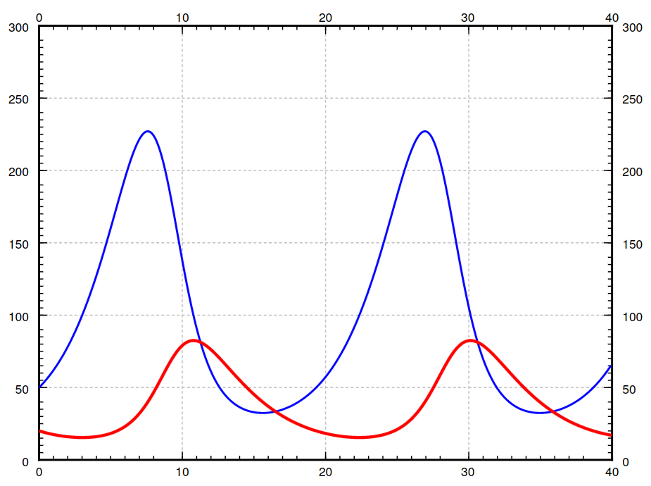
Example

Solve the Lotka-Voltera system $$ \begin{array}{l} x_1'=(0.4-0.01x_2)x_1\\ x_2'=(0.003x_1-0.3)x_2\\ \end{array} $$ using Runge-Kutta methods with initial conditions:

$\displaystyle x_1(0)=$, $\displaystyle x_2(0)=$

	Prey		Predator		Phase Plane Trajectory
$x_1$		$x_2$		$x_2$
	$t$		$t$		$x_1$

Phase Portrait of Lotka-Volterra System

$ \begin{array}{l} \mbox{System}\\ x'=(0.4-0.01y)x\\ y'=(0.003x-0.3)y\\ \\ \mbox{Direction Field}\\ \langle (0.4-0.01y)x,(0.003x-0.3)y\rangle\\ \\ \mbox{Slope Field}\\ \displaystyle \frac{dy}{dx}=\frac{(0.003x-0.3)y}{(0.4-0.01y)x} \end{array} $

Existence and Uniqueness: Picard’s Theorem for First-Order Systems.

If for every $i\in \{1, 2, \ldots , n\},$ and every $k\in \{1, 2, \ldots , n\}$ each $f_j$ is continuous and the derivative $\displaystyle \frac{\partial f_j}{\partial x_k}$ exists and is continuous near some $(a_1,a_2,\ldots,a_n)$, then a solution to the system with initial conditions $$ x_1'=f_1(x_1,x_2,\cdots, x_n,t),\,\,\,\,\,x_1(t_0)=a_1\\ x_2'=f_2(x_1,x_2,\cdots, x_n,t),\,\,\,\,\,x_2(t_0)=a_2\\ \vdots\\ x_n'=f_n(x_1,x_2,\cdots, x_n,t),\,\,\,\,\,x_n(t_0)=a_n $$ exists (at least for $t$ in some small interval) and is unique.

Picard is watching you.