As we have seen already, some equations we simply cannot solve.
Not all hope is lost though when this happens. (It happens a lot!)
We've seen methods which enable us to understand the overall qualitative behavior of solutions to equations (slope fields and phase-line methods.)
However, if we need a more exact estimate of a future state, we'll need other techniques.
Euler's Method
Recall that by knowing the slope of the tangent line to a function $f(x),$ we can approximate the the value of $f(x)$ near a point $(x_0,f(x_0))$ by using the linearization of $f(x).$ $$ \Delta y=y-f(x_0)\approx f'(x_0)(x-x_0)=hf'(x_0) $$
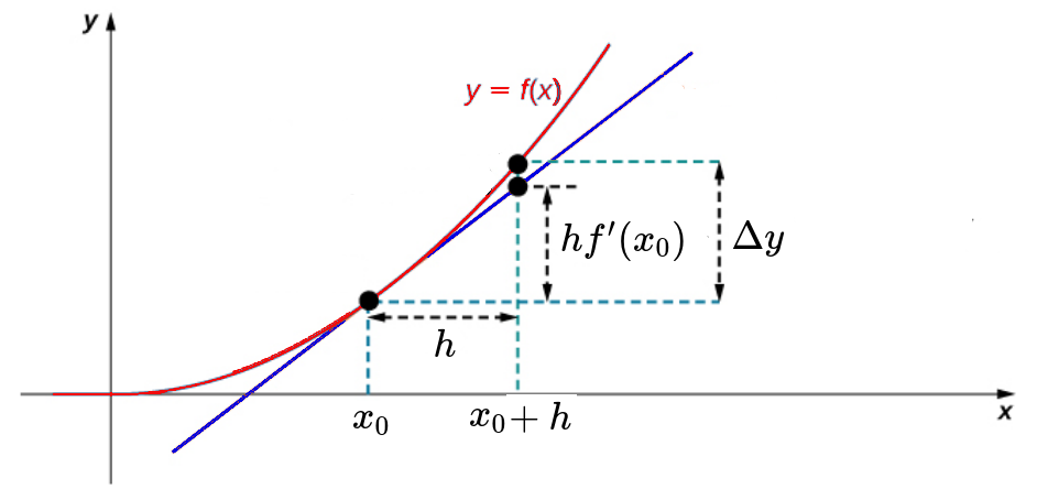
This, idea is the basis of Euler's Method.
Euler's Method
Consider a generic first-order initial value problem $$ y'=f(x,y), \,\,\,\,\,\, y(x_0)=y_0 $$ The expression $f(x,y)$ gives us the slope of $y(x)$ at every point $x.$
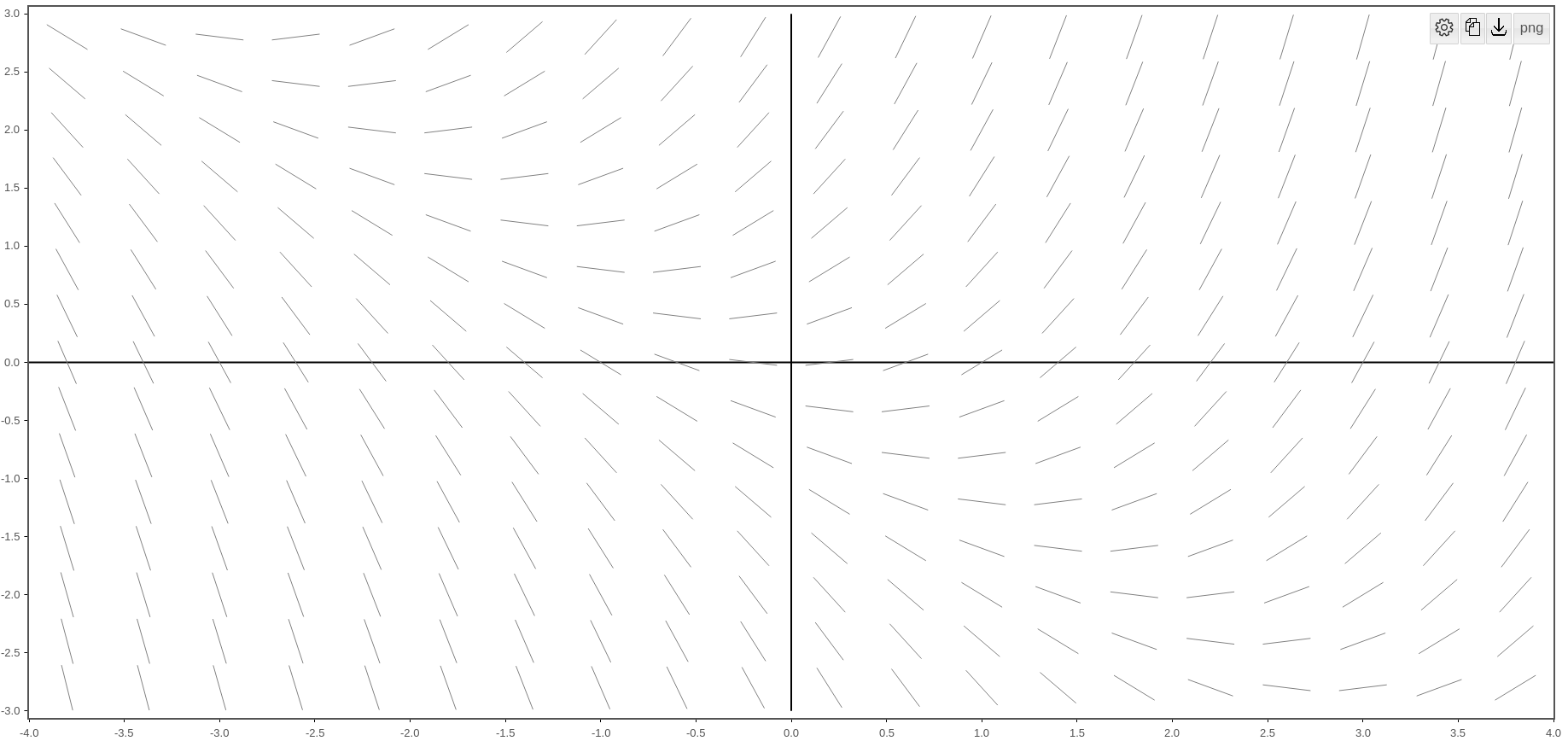
Euler's Method
We suppose a solution $y$ exists to $ y'=f(x,y), \,\,\, y(x_0)=y_0 $
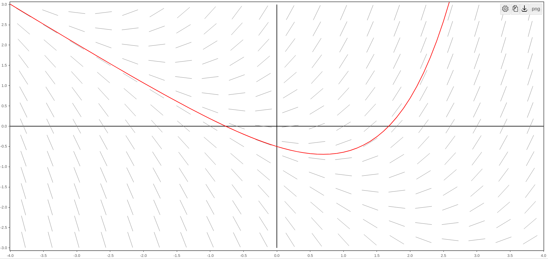
Euler's Method
We then specify our initial point $(x_0,y_0)$ and use the linearization (tangent line) of $y$ to guess the next value of $y.$
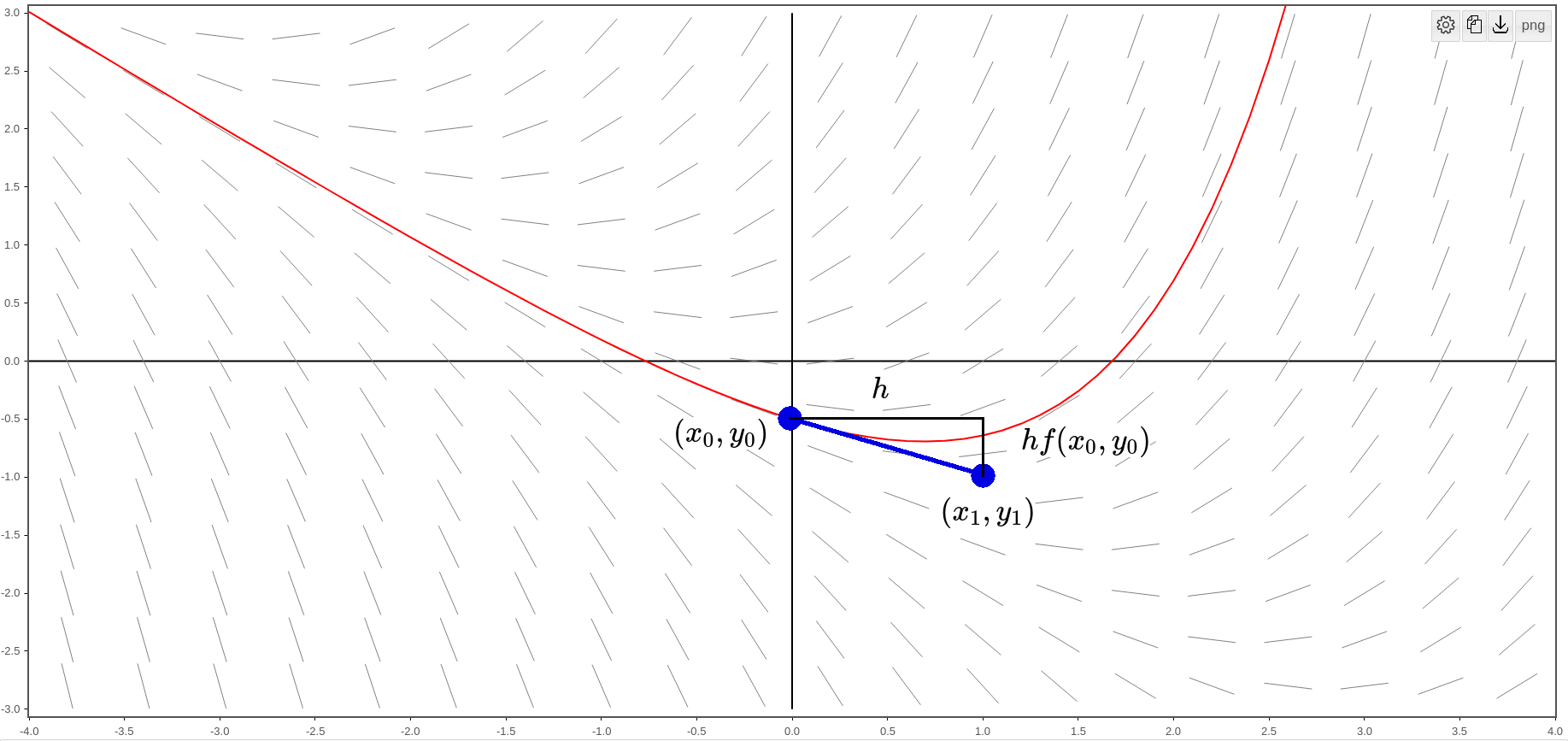
As we can see, the next point $(x_1,y_1)$ is a little bit off the exact curve, and that's okay, as long as it's close to the exact value.
We also see that $y_1=y_0+hf(x_0,y_0).$
Euler's Method
We use the slope given by $f(x,y)$ at $(x_1,y_1)$ to determine the next approximate value of $y$ at a point $(x_2,y_2).$
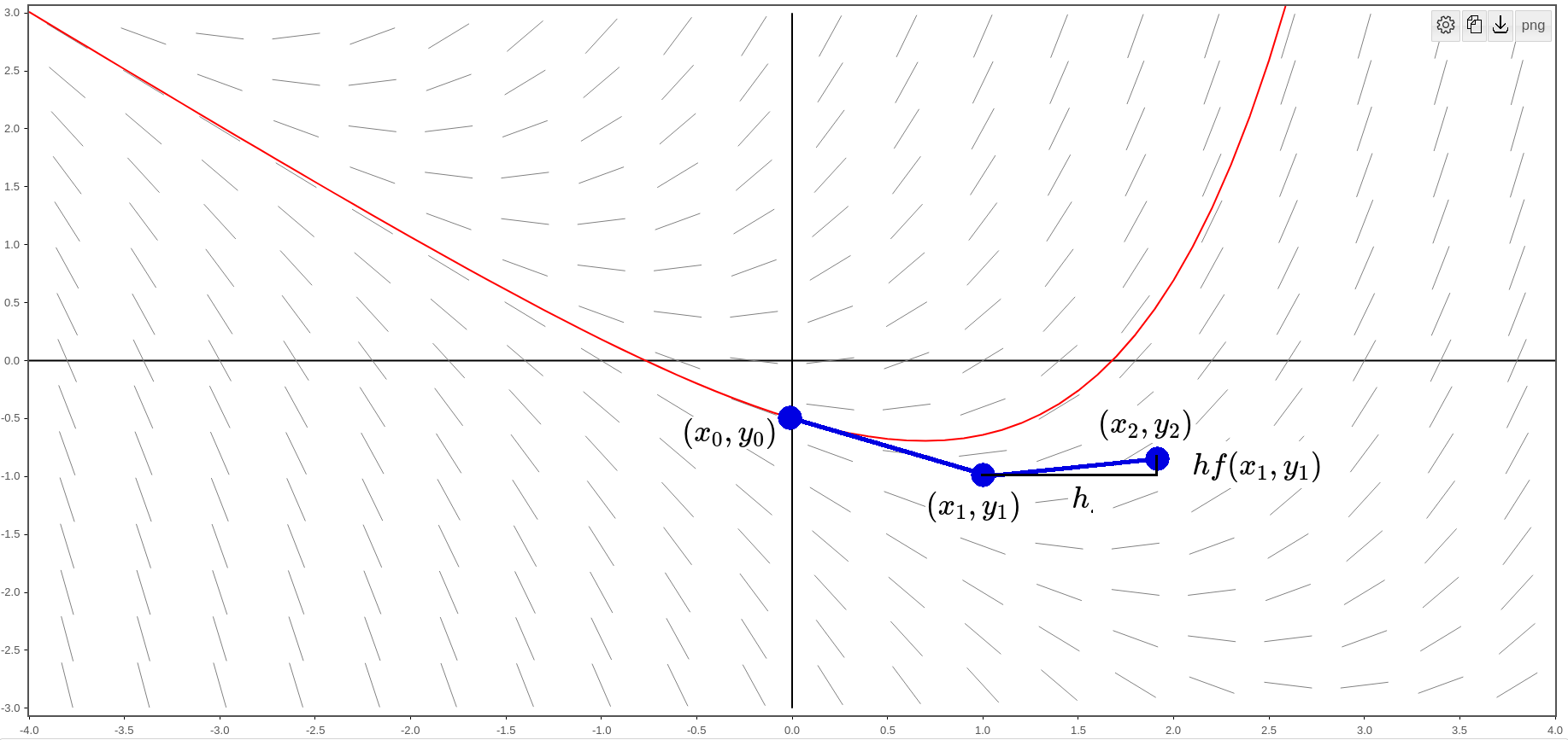
We see that $y_2=y_1+hf(x_1,y_1).$
Euler's Method
We then use the slope given by $f(x,y)$ at $(x_2,y_2)$ to determine the next approximate value of $y$ at a point $(x_3,y_3).$
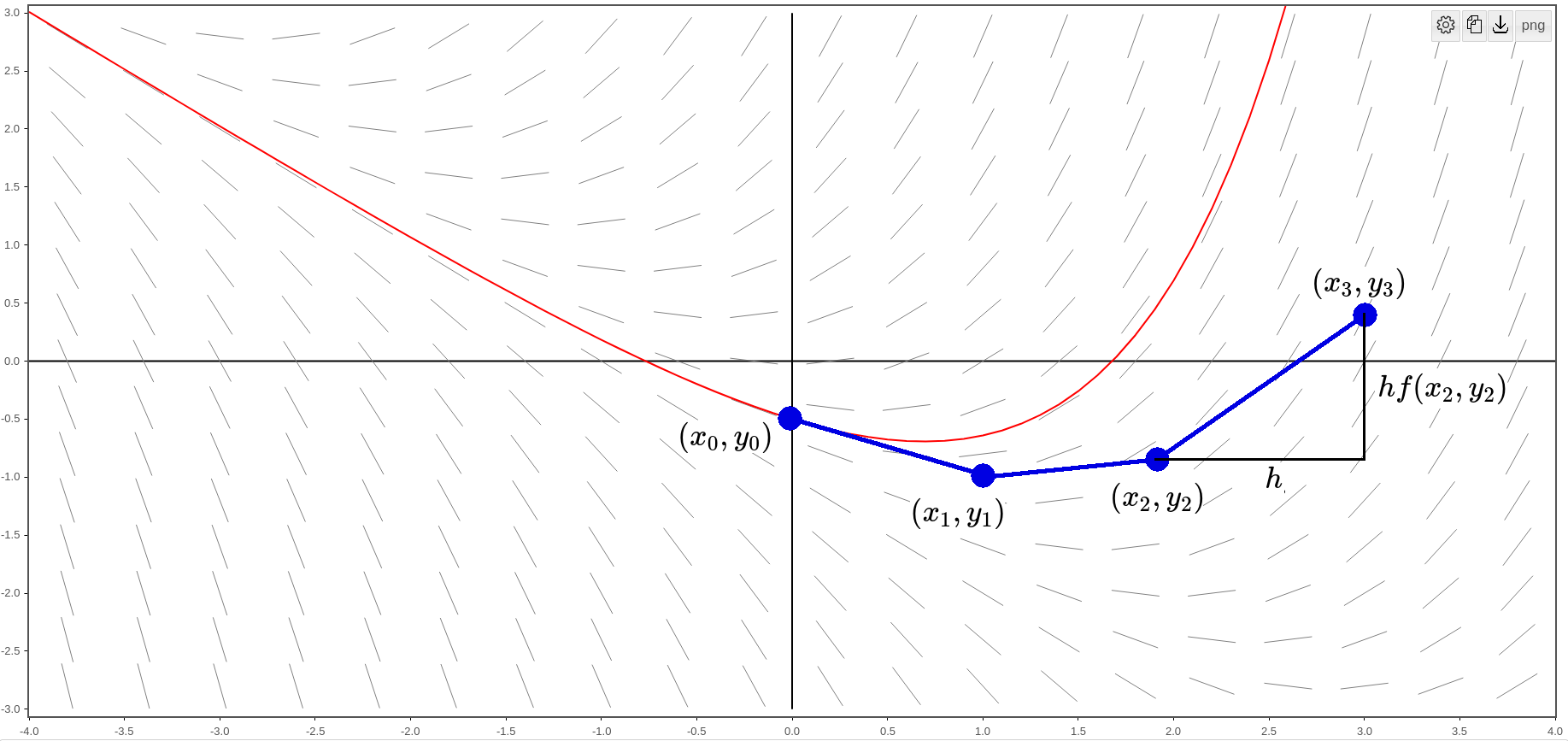
We see that $y_3=y_2+hf(x_2,y_2).$
Euler's Method
And we repeat the process until we are at the future state we want to predict.

The idea is the approximation is close to the true value of $y.$
From the above, we saw that we started at an initial point $(x_0,y_0)$ and computed $$ \begin{array}{lll} \displaystyle &\displaystyle x_{1}=x_0+h &\mbox{}\\ \displaystyle &\displaystyle y_{1}=y_0+hf(x_0,y_0) &\mbox{}\\ \end{array} $$ and then $$ \begin{array}{lll} \displaystyle &\displaystyle x_{2}=x_1+h &\mbox{}\\ \displaystyle &\displaystyle y_{2}=y_1+hf(x_1,y_1) &\mbox{}\\ \end{array} $$ and then $$ \begin{array}{lll} \displaystyle &\displaystyle x_{3}=x_2+h &\mbox{}\\ \displaystyle &\displaystyle y_{3}=y_2+hf(x_2,y_2) &\mbox{}\\ \end{array} $$ Can you see the pattern?
Euler's Method
Suppose we have the initial value problem $$ y'=f(x,y), \,\,\,\,\,\, y(x_0)=y_0 $$ First, choose a step size $h.$ Then compute $$ \begin{array}{lll} \displaystyle &\displaystyle x_{n+1}=x_n+h &\mbox{}\\ \displaystyle &\displaystyle y_{n+1}=y_n+hf(x_n,y_n) &\mbox{}\\ \end{array} $$ If all goes well, the values $(x_n,y_n)$ should lie close to the true solution $y(x).$
Example
Consider the initial value problem. $$ y'=x+y, \,\,\,\,\,\, y(0)=-0.5 $$ Use Euler's Method to approximate $y(1)$ with step sizes $h=0.1.$
| $\displaystyle x_n$ | $y_n$ |
$\displaystyle h=$,
$\displaystyle \,\,\,\,\,\,\,\,y(0)=$
Euler's Method with Decreasing Step Sizes
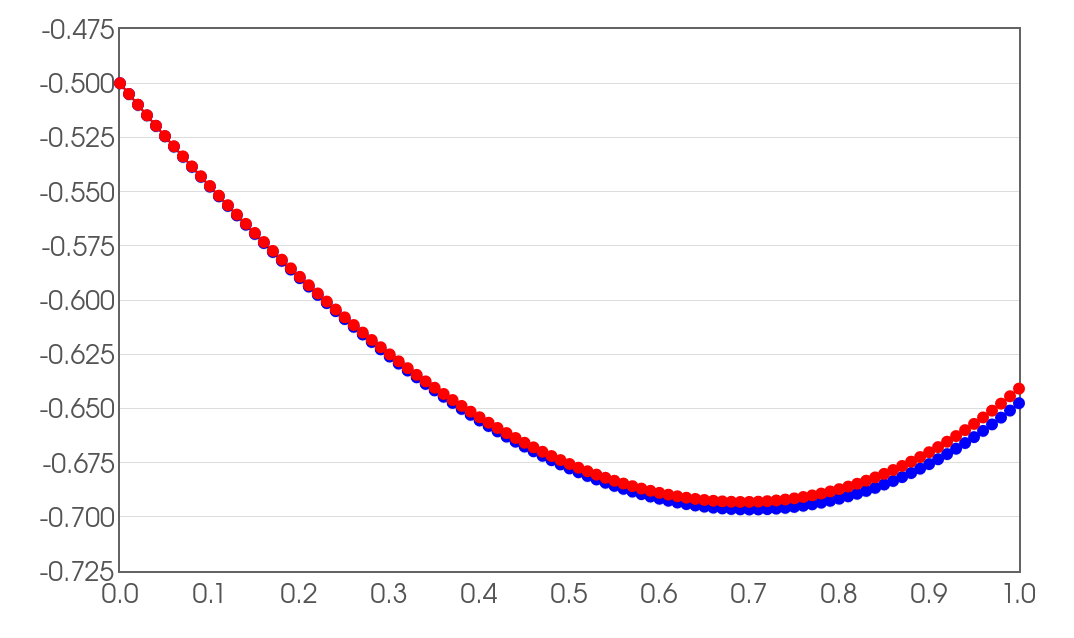
Euler-method approximation of $y(1)$ with step sizes $h=0.1,$ $0.05,$ and $0.01.$
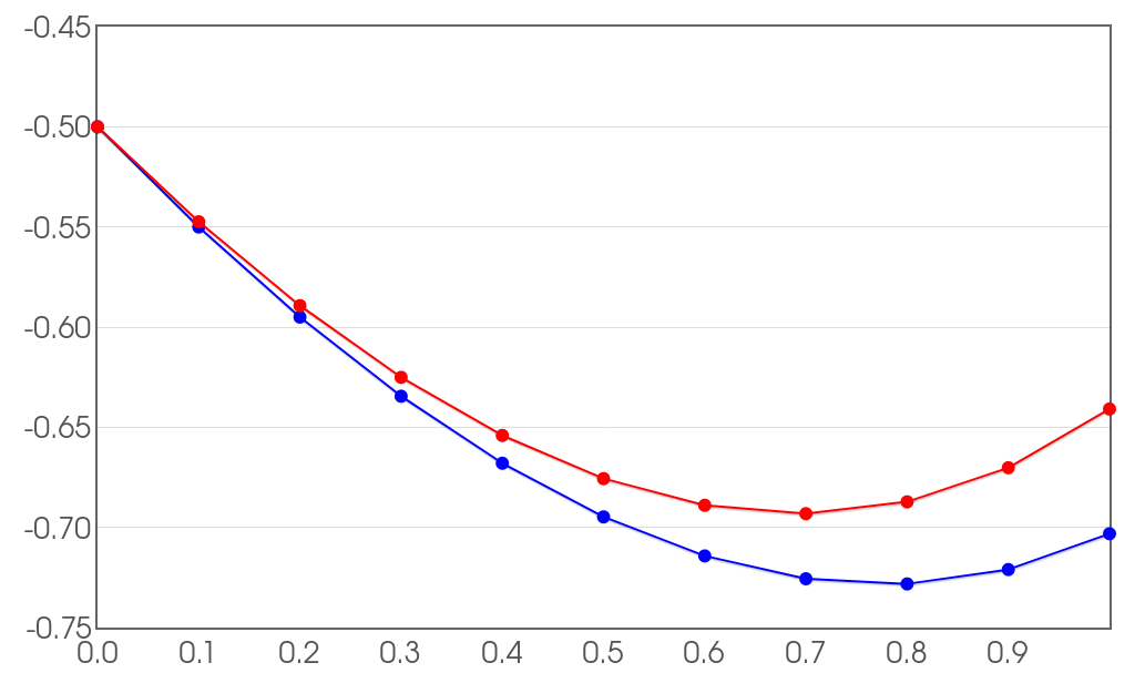
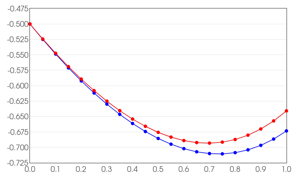
Euler-Method Error
Let's make a table of errors for the above for our estimation of $y(1)$ for varying step sizes $h.$ $$ \begin{array}{lll} h & \mbox{Error}=|y(1)-y_n| & \frac{\mbox{Current Error}}{\mbox{Previous Error}}\\ 1 & 0.35914091422952255 & \\ 0.5 & 0.23414091422952255 & 0.651947202\\ 0.25 & 0.13843778922952255 & 0.59125843\\ 0.125 & 0.0762486572543486 & 0.550779218\\ 0.0625 & 0.04017666554622257 & 0.526916368\\ 0.03125 & 0.02064584954043136 & 0.513876631\\ 0.015625 & 0.010468437946972942 & 0.50704806\\ \end{array} $$ Question: Each time we halve the step size $h,$ approximately what happens to the error of our approximation?
Big Question
Can we devise a scheme which is better at approximating solutions than Euler's Method?
Big Answer

The Runge-Kutta Method
For the initial value problem $$ y'=f(x,y), \,\,\,\,\,\, y(x_0)=y_0 $$ choose a step size $h.$ Then compute $$ \begin{array}{lll} \displaystyle &\displaystyle x_{n+1}=x_n+h &\mbox{}\\ \displaystyle &\displaystyle y_{n+1}=y_n+h\frac{k_1+2k_2+2k_3+k_4}{6} &\mbox{}\\ \end{array} $$ where $$ \begin{array}{lll} \displaystyle &\displaystyle k_1=f(x_n,y_n) &\mbox{}\\ \displaystyle &\displaystyle k_2=f\left(x_n+\frac{1}{2}h,y_n+\frac{1}{2}hk_1\right) &\mbox{}\\ \displaystyle &\displaystyle k_3=f\left(x_n+\frac{1}{2}h,y_n+\frac{1}{2}hk_2\right) &\mbox{}\\ \displaystyle &\displaystyle k_4=f(x_n+h,y_n+hk_3) &\mbox{}\\ \end{array} $$
Example
Consider the initial value problem. $$ y'=x+y, \,\,\,\,\,\, y(0)=-0.5 $$ Use the Runge-Kutta Method to approximate $y(0.1)$ with step sizes $h=0.1.$
The initial value is $(x_0,y_0)=(0,-0.5).$ Then, since $h=0.1,$
$$
\begin{array}{lll}
\displaystyle &\displaystyle k_1=f(x_0,y_0)=f(0,-0.5)=0+(-0.5)=-0.5 &\mbox{}\\
\displaystyle &\displaystyle k_2=f\left(x_0+\frac{1}{2}h,y_0+\frac{1}{2}hk_1\right)=f\left(0+\frac{1}{2}\cdot 0.1,-0.5+\frac{1}{2}\cdot 0.1 \cdot (-0.5) \right)=f(0.05,-0.525)=-0.475 &\mbox{}\\
\displaystyle &\displaystyle k_3=f\left(x_0+\frac{1}{2}h,y_0+\frac{1}{2}hk_2\right)=f\left(0+\frac{1}{2}\cdot 0.1,-0.5+\frac{1}{2}\cdot 0.1 \cdot (-0.475) \right)=f(0.05,-0.52375)=-0.47375 &\mbox{}\\
\displaystyle &\displaystyle k_4=f(x_0+h,y_0+hk_3)=f(0+0.1,-0.5+0.1\cdot (-0.47375))=f(0.1,-0.547375)=-0.447375 &\mbox{}\\
\end{array}
$$
and we have
$$
\begin{array}{lll}
\displaystyle &\displaystyle x_{1}&=x_0+h=0+0.1\\
\displaystyle &\displaystyle &\mbox{}\\
\displaystyle &\displaystyle y_{1}&=\displaystyle y_0+h\frac{k_1+2k_2+2k_3+k_4}{6}\\
\displaystyle &\displaystyle &=\displaystyle-0.5+0.1\cdot \frac{-0.5+2(-0.475)+2(-0.47375)+(-0.447375)}{6}\\
\displaystyle &\displaystyle &=\displaystyle-0.5474145833\\
%\displaystyle &\displaystyle y_{1}=y_0+h\frac{k_1+2k_2+2k_3+k_4}{6}=-0.5+0.1\cdot \frac{-0.5+2(-0.475)+2(-0.47375)+(-0.447375)}{6}=-0.5474145833 &\mbox{}\\
\end{array}
$$
The Runge-Kutta Method
$\displaystyle h=$,
$\displaystyle \,\,\,\,\,\,\,\,y(0)=$
Comparison Euler vs. Runge-Kutta
The Euler-Method (left) and Runge-Kutta-Method (right) approximation of $y(1)$ with step size $h=0.1.$

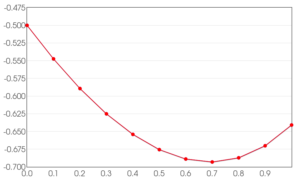 $\mbox{Error}=|y(1)-y_{10}|=0.06226968417952239\,\,\,\,\,\,\,\,\,\,\,\,\,\,\mbox{Error}=|y(1)-y_{10}|=0.0000010421619396350223$
Runge-Kutta Method Error
Let's make a table of errors for the above for our estimation of $y(1)$ for varying step sizes $h.$ $$ \begin{array}{lll} h & \mbox{Error}=|y(1)-y_n| & \frac{\mbox{Current Error}}{\mbox{Previous Error}}\\ 1 & 0.004974247562855916 & \\ 0.5 & 0.0004678185263975454 & 0.094048099 \\ 0.25 & 0.000035944628861139805 & 0.076834556\\ 0.125 & 0.0000024920211555423677 & 0.069329445\\ 0.0625 & 0.00000001640592300899968 & 0.0658338\\ 0.03125 & 0.0000000010523925619843055 & 0.064147111\\ 0.015625 & 0.00000000006663605223167224 & 0.063318627\\ \end{array} $$ Question: Any guesses for the exact factor by which the error is reduced?
The Order of a Numerical Approximation Method
Suppose we reduce the step size $h$ of of a numerical approximation method by one half.
The order of a numerical approximation method is the approximate number of halvings of the error when the step size is reduced by one half.
Example: Euler's Method is an $\color{magenta}{1}$st-order approximation method since the error halved about once when step size is decreased by half. That is, $\displaystyle \left(\frac{1}{2}\right)^\color{magenta}{1}=\frac{1}{2}=0.5$
Example: The Runge-Kutta Method is an $\color{magenta}{4}$th-order approximation method since the error is halved about four times when the step size is decreased by half. That is, $\displaystyle \left(\frac{1}{2}\right)^\color{magenta}{4}=\frac{1}{16}=0.0625$.
A Note About Error
Please keep in mind that we've been able to compute the error since we can compute the exact solution.
In practice, when we don't have an exact solution, this isn't possible.
In fact, if we could find the exact error, then we could find the exact value!
Notes on Numerical Stability
There are conditions under which a numerical scheme can become unstable.
Example: Consider the initial value problem $$y'=-2xy, \,\,\,\, y(0)=1.$$ Run Euler's Method with step sizes $h=0.1,$ $h=0.5$ and $h=0.51.$
$\displaystyle h=$,
$\displaystyle \,\,\,\,\,\,\,\,y(0)=$
Notes on Numerical Stability
Both Euler's Method and the Runge-Kutta Method (a.k.a. $\mbox{RK4}$) are prone to instability under certain conditions.
Some Things to Consider When Using Numerical Methods
Stability: As we have seen, be mindful of situations when a numerical scheme can become unstable. Although increasing step size might reduce the computation time, it can result in instability (as we have seen). Also, some equations either need an impractically small step size for a stable solution, or the scheme won't stabilize for any step size. Equations which are mired in these kinds of difficulties are called stiff equations.
Computational Cost: Although decreasing step size can reduce both computational error and the possibility of numerical instability, it will certainly take longer to compute the quantity you are interested in.
Round-Off Errors: Decreasing step size is not a guarantee of better results. Depending on how your machine implements floating-point arithmetic, decreasing the step size beyond a certain threshold can make errors even worse.
Finally, the author of our text also notes,
"In the worst case, the numerical computations might be giving us bogus numbers that look like a correct answer. Just because the numbers seem to have stabilized after successive halving, does not mean that we must have the right answer."
In Summary
Using numerical methods involves a trade off between computational error, time of computation, and issues of stability.
Finding that sweet spot will depend on the situation you are faced with.
One Last Note
Euler's Method is a generalization of a left-hand Riemann sum.
$\mbox{RK4}$ is a generalization of Simpson's method for approximating integrals.
In fact, if the solution to an equation is a simple integral, that is $$y'=f(x)$$ then Euler's method becomes a left-hand Riemann sum, and $\mbox{RK4}$ reduces down to Simpson's Method.