Let $x$ be a dependent variable which depends on $t.$
An equation is autonomous if $x'$ can be expressed solely in terms of $x.$
That is, autonomous equations have the form $$ x'=f(x) $$
Examples of Autonomous Equations
$\displaystyle \frac{dP}{dt}=kP,$ uninhibited population growth (Malthusian growth)
$\displaystyle \frac{dP}{dt}=kP\left(1-\frac{P}{K}\right),$ limited population growth (logistic growth)
$\displaystyle \frac{dT}{dt}=k(T-T_a)$ Newton's Law of Cooling
$\displaystyle -\frac{d[A]}{dt}=k[A]^n,$ equation describing the concentration of a reactant in an $n$th order reaction
The above are all autonomous since the dependent variable does not depend in any way upon the independent variable $t.$
Example: Consider a population of critters modelled by the logistic equation $$ x'=0.1x(5-x) $$
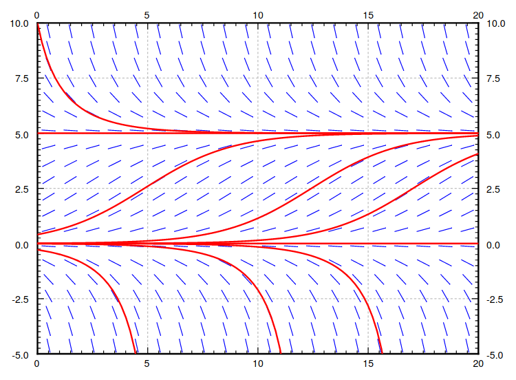
The carrying capacity of this population of critters is $5.$
This could mean $5$ million individuals, it could mean $5$ grams of a certain bacterial culture.
The distinction is not important. What is important is that the logistic equation is a reasonable model of limited population growth.
Example: Consider a population of critters modelled by the logistic equation $$ x'=0.1x(5-x) $$


The thing to note about the slope field of this (autonomous!) equation is that the slopes do not change with $t.$ They only change with $x'.$
Thus we may capture the qualitative dynamics of the situation with a figure much simpler than a slope field.
Example: Consider a population of critters modelled by the logistic equation $$ x'=0.1x(5-x) $$
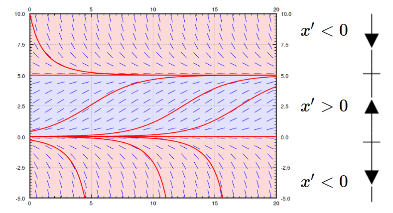
Instead of a slope field, we use a phase line seen above on the right.
What really matters here is when $x'=f(x)$ is positive negative, or $0.$
Finding the Phase Line
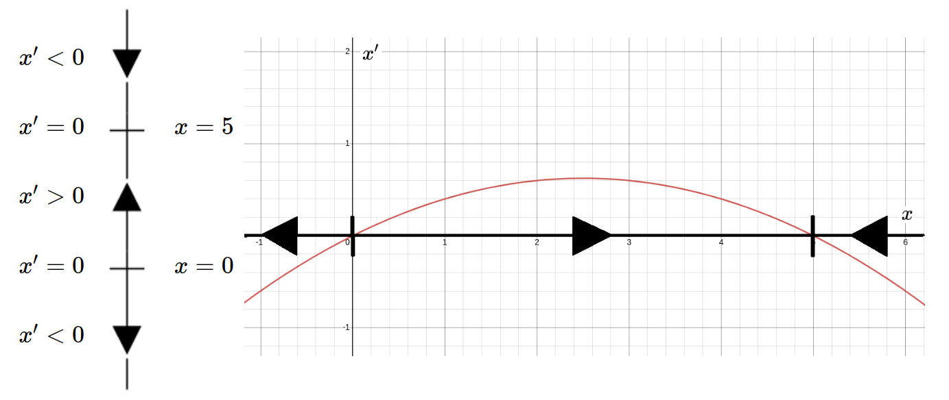
Good News: Finding the phase line is relatively simple.
Consider the phase line for the logistic equation $x'=0.1x(5-x)$ and the graph of $x'$ versus $x.$
Critical Points
Consider an autonomous equation $$ x'=f(x) $$ A critical point is a value of $x$ for which $f(x)=0.$
Critical points correspond to equilibrium solutions which are constant solutions ($x'=0$ for all $t$).
A critical point is called stable if any solution near its corresponding equilibrium solution, say $x=A,$ tends toward $A$ in the sense that $$\displaystyle \lim_{t\rightarrow \infty} x(t)=A$$ A critical point is called unstable if it is not stable.
Example
The critical points of the equation $x'=0.1x(5-x)$ are $x=0$ and $x=5.$

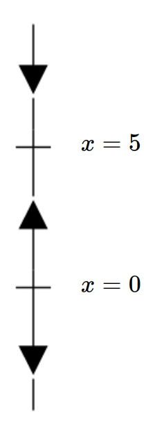
Since solutions near $x=5$ tend toward $5$ in the sense that $\displaystyle \lim_{t\rightarrow \infty} x(t)=5,$ the critical point $x=5$ is stable.
On the other hand, the point $x=0$ is unstable since there are values nearby who solutions get pulled somewhere else.
Perturbations
A solution near an equilibrium solution is called a perturbation.
We may rephrase our definition of stability of a critical point by saying that it stable if a small perturbation away from it corresponding equilibrium solution $x=A$ in either direction results in a solution which tends toward $x=A$ as $t\rightarrow \infty.$
On the other hand, for an unstable critical point, perturbations on at least one side of the corresponding equilibrium solution $x=A$ will get pulled off to some other place as $t\rightarrow \infty.$
Example
The critical points of the equation $x'=0.1x(5-x)$ are $x=0$ and $x=5.$


Since $x=5$ is a stable critical point, small perturbations away from $x=5$ result in solutions which still tend toward $5$ as $t\rightarrow \infty.$
On the other hand, since $x=0$ is an unstable critical point, perturbations above and below the equilibrium solution the equilibrium solution $x=0$ get pulled off to some other place as $t\rightarrow \infty.$
Classifying Critical Points
Good News: Not only is finding the phase line a relatively simple process, classifying critical points is easily accomplished by simply looking at the phase line.
 | 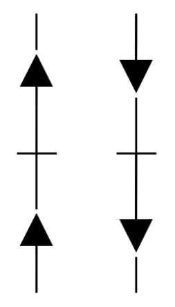 |  |
| stable | semi-stable (node) | unstable |
Example
The critical points of the equation $x'=0.1x(5-x)$ are $x=0$ and $x=5.$

$x=5$ is a stable critical point.
$x=0$ is an unstable critical point,
Finally, A New Example!
Find and classify the critical points of for the autonomous equation $$ x'=(x-1)(x-2)(x-3) $$
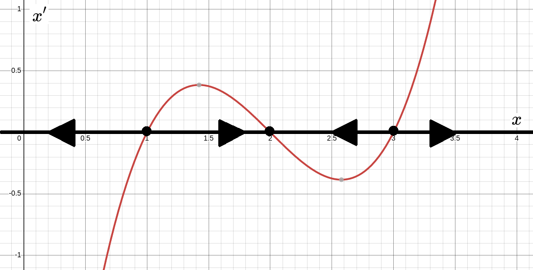
The critical points occur where $x'=f(x)=(x-1)(x-2)(x-3)=0.$
That is, the critical points are $x=1,$ $x=2,$ and $x=3.$
Graphing $x'$ versus $x,$ we have
The phase line diagram is then
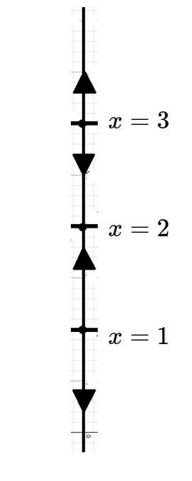
We see that $x=2$ is a stable critical point, whereas, $x=1$ and $x=3$ are unstable critical points.
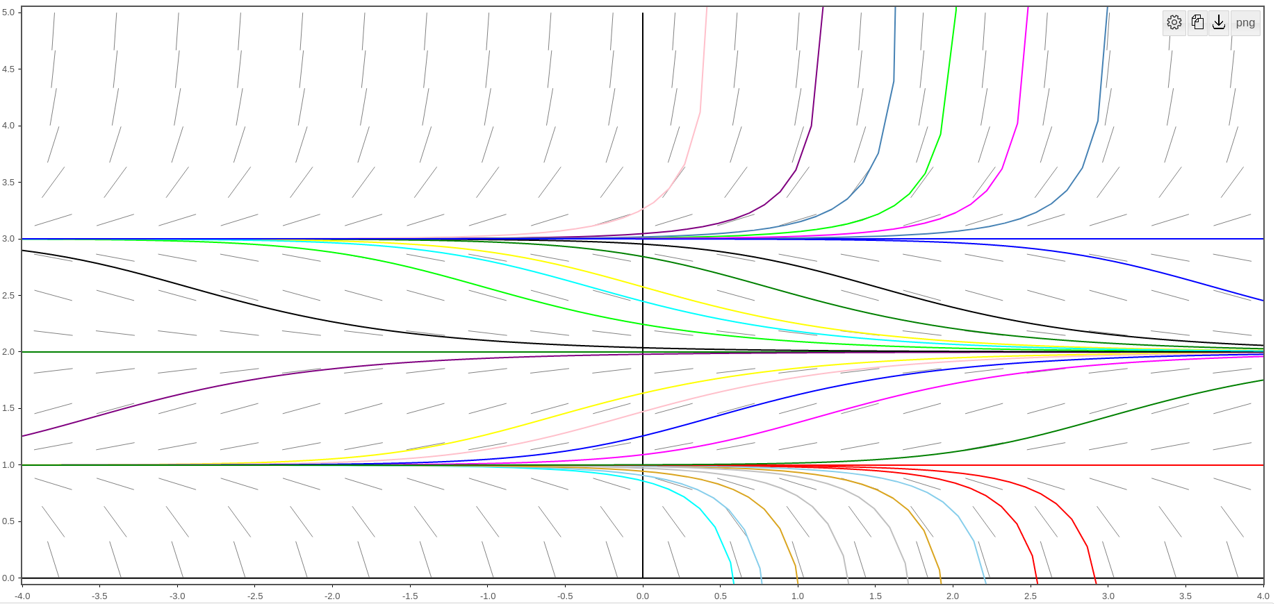
Although the slope field is generally overkill for understanding the qualitative behavior of autonomous equations, it's still illuminating to see the corresponding slope field with solutions near the equilibrium solutions with the corresponding phase line diagram.

That is, the critical points are $x=1,$ $x=2,$ and $x=3.$
Graphing $x'$ versus $x,$ we have

The phase line diagram is then

We see that $x=2$ is a stable critical point, whereas, $x=1$ and $x=3$ are unstable critical points.
Although the slope field is generally overkill for understanding the qualitative behavior of autonomous equations, it's still illuminating to see the corresponding slope field with solutions near the equilibrium solutions with the corresponding phase line diagram.


Example: Logistic Growth with Harvesting/Culling
Let's suppose we have a population of critters whose dynamics are governed by the equation $$ x'=\frac{1}{3200}x(1500-x) $$ Suppose hunters are allowed to harvested/cull the population by a constant amount $h$ critters per year.
What is the smallest value of $h$ which would cause the population to be eradicated?
The differential equation which accounts for the yearly harvesting is
$$
x'=\frac{1}{3200}x(1500-x)-h
$$
The critical points of this equation are are those values of $x$ for which
$$
x'=f(x)=\frac{1}{3200}x(1500-x)-h=0
$$
Then
$$
\begin{array}{lll}
&\displaystyle x(1500-x)-3200h=0&\mbox{}\\
\implies &\displaystyle -x^2+1500x-3200h=0&\mbox{}\\
\implies &\displaystyle x^2-1500x+3200h=0&\mbox{}\\
\implies &\displaystyle x=\frac{1500\pm\sqrt{1500^2-12800h}}{2}&\mbox{}\\
\implies &\displaystyle x=750\pm\sqrt{562500-3200h}&\mbox{}\\
\end{array}
$$
The two potential equilibrium solutions are, therefore,
$$x=750+\sqrt{562500-3200h}\,\,\,\,\mbox{}\,\,\,\, x=750-\sqrt{562500-3200h}$$
We see that if $h$ is small enough so that $562500-3200h\gt 0,$ we have two equilibrium solutions.
On the other hand, if the hunters harvest too many critters, the equilibrium solutions disappear since $562500-3200h\lt 0.$
In fact, the "tipping point" for this population occurs where $\displaystyle h=\frac{562500}{3200}\approx 175.78.$
If the hunters harvest more than $175$ critters, then the population is doomed.
To more fully appreciate this example, lets look at the phase line diagrams for varying values of $h.$
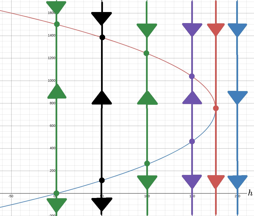
The above bifurcation diagram shows how the critical points of the equation vary with $h.$
The phase lines correspond to $h=0, 50, 100, 150, 176,$ and $200.$
In short, any harvesting above $175$ critters per year will annihilate the population.
On the other hand, if the hunters harvest too many critters, the equilibrium solutions disappear since $562500-3200h\lt 0.$
In fact, the "tipping point" for this population occurs where $\displaystyle h=\frac{562500}{3200}\approx 175.78.$
If the hunters harvest more than $175$ critters, then the population is doomed.
To more fully appreciate this example, lets look at the phase line diagrams for varying values of $h.$

The above bifurcation diagram shows how the critical points of the equation vary with $h.$
The phase lines correspond to $h=0, 50, 100, 150, 176,$ and $200.$
In short, any harvesting above $175$ critters per year will annihilate the population.
A Few More Fun Facts
Qualitative analysis of differential equations like slope fields as well as the above phase-line analysis can yield great insight into the dynamics of a situation without having to solve any equations.
Notice that we haven't solved a single DE during this entire section!
Due to their relative simplicity, autonomous equations and phase-line analysis can afford us a great deal of information in exchange for very little effort.
Lest we believe that this kind of analysis isn't really all that practical, consider the examples of autonomous equations we saw earlier involving not only population dynamics, but also temperature dynamics (Newton's Law of Cooling) and chemical equilibria.