An equation involving an unknown function and its derivatives is known as a differential equation.
As we shall see, differential equations appear in a diversity of disciplines! From physics, to chemistry, biology, epidemiology, psychology, sociology (the spread of information).
Example
The equation $$ \frac{dx}{dt}+x=2\cos t $$ is an example of a differential equation since it involves an unknown function $x(t)$ and its derivative $\displaystyle \frac{dx}{dt}.$
Differential Equations are Workhorses of Applied Mathematics!
As we shall see a we proceed through the course, many applied problems are stated as an equation involving some unknown function $y(x)$ and its derivatives $\displaystyle \frac{dy}{dx},$ $\displaystyle \frac{d^2y}{dx^2},$ $\displaystyle \frac{d^3y}{dx^3}...$
Fun Fact
Since second-term (integral) calculus, we have been solving differential equations, we just didn't know it!
Finding an antiderivative of $f(x)$ amounts to answering the question, "what function(s) $y$ give back $f(x)$ when we take their derivative?"
That is, we are solving a very basic differential equation $$\frac{dy}{dx}=f(x).$$
Example
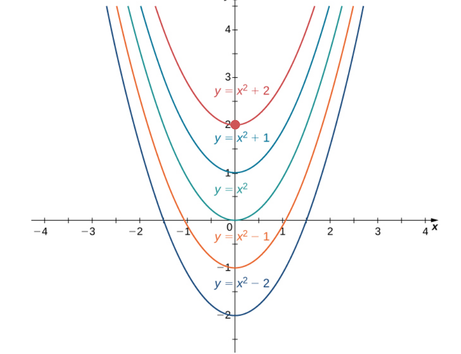
The family of antiderivatives $\displaystyle y=\int 2x \,dx=x^2+C$ solves the differential equation $$\frac{dy}{dx}=2x.$$
Initial Value Problems
In applications, it is very common to find a solution to differential equation that satisfies a particular condition called an initial condition.
For example, it might be that we need a function which satisfies the differential $\displaystyle \frac{dy}{dx}=2x$ as well as an initial condition $y(0)=2.$
Initial Value Problems
Example: Solve the initial value problem $\displaystyle \frac{dy}{dx}=2x,$ $y(0)=2.$

We can see that the solution $y=x^2+2$ satisfies both the differential equation and the initial condition $y(0)=2.$
Some Examples
Some differential equations from physics you might already be familiar with include $$ \begin{array}{lll} \displaystyle &\displaystyle \frac{ds}{dt}=v(t) &\mbox{Velocity is the derivative of postion.}\\ \displaystyle &\displaystyle \frac{dv}{dt}=a(t) &\mbox{Acceleration is the derivative of velocity.}\\ \displaystyle &\displaystyle \frac{d^2s}{dt^2}=a(t) &\mbox{Acceleration is the second derivative of postion.}\\ \displaystyle &\displaystyle \frac{d^2s}{dt^2}=-g &\mbox{The equation for free fall neglecting air resistance.}\\ \end{array} $$
A Differential Equation You've Probably Not Seen
Although you may have seen some differential equations already, you've likely never encountered anything like the following in previous courses: $$ \frac{dx}{dt}+x=2\cos t $$ Fun Fact: The above equation qualitatively describes how the temperature of a cooling body changes with a fluctuating ambient temperature.
Verifying Solutions
For the differential equation $$ \frac{dx}{dt}+x=2\cos t $$ show that $ x(t)=\cos t + \sin t+Ce^{-t} $ is a solution where $C$ can be any constant.

$$
\begin{array}{lll}
\displaystyle \frac{dx}{dt}+x&\displaystyle=\frac{d}{dt}(\cos t + \sin t+Ce^{-t})+\cos t + \sin t+Ce^{-t} &\mbox{}\\
\displaystyle &\displaystyle=-\sin t+\cos t-Ce^{-t}+\cos t + \sin t+Ce^{-t} &\mbox{}\\
\displaystyle &\displaystyle=2\cos t &\mbox{}\\
\end{array}
$$
Satisfying Initial Conditions
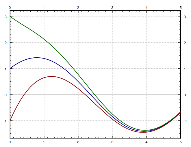
We saw that $ x(t)=\cos t + \sin t+Ce^{-t} $ is a solution to the equation $$ \frac{dx}{dt}+x=2\cos t $$ For what value of $C$ is the initial condition $x(0)=3$ satisfied?

$$
\begin{array}{lll}
&\displaystyle x(0)=3&\mbox{}\\
\implies &\displaystyle \cos 0 + \sin 0+Ce^{-0}=3&\mbox{}\\
\implies &\displaystyle 1 +C=3&\mbox{}\\
\implies &\displaystyle C=2&\mbox{}\\
\end{array}
$$
Thus, $x(t)=\cos t + \sin t+2e^{-t}$ satisfies the equation and initial condition $x(0)=3.$
Some Vocab
For the equation $$ \frac{dx}{dt}+x=2\cos t $$ The family of solutions $x(t)=\cos t + \sin t+Ce^{-t}$ where $C$ can be any constant is called the general solution.
When a value of $C,$ is specified a solution is called a particular solution.
For example, the solution satisfying the initial condition $x(0)=3,$ that is $x(t)=\cos t + \sin t+2e^{-t},$ is a particular solution.
Population Growth
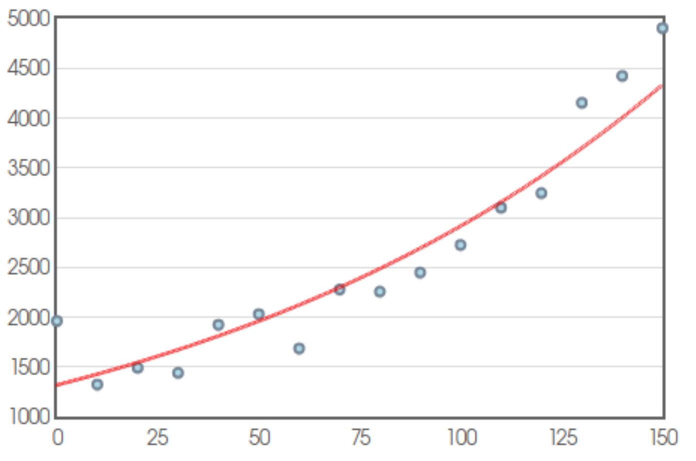
The population $P$ at time $t$ of Mr. Holt's hometown can be modelled by the differential equation $$ \frac{dP}{dt}=0.008P $$ whose general solution is $P=Ce^{0.008t}.$


If the initial population of the model (the red curve) in $1860$ (year $0$) was $1318$ people find $P(t).$ What is the estimated population for $2020?$ (year $160$)
Since $P=Ce^{0.008t}$ and the initial condition is $P(0)=1318,$ we have
$$
\begin{array}{lll}
&\displaystyle P(0)=1318&\mbox{}\\
\implies &\displaystyle Ce^{0.008\cdot 0}=1318&\mbox{}\\
\implies &\displaystyle C=1318&\mbox{}\\
\end{array}
$$
Thus, $P=1318e^{0.008t}.$
We then have that $$ \begin{array}{lll} \displaystyle P(160) &\displaystyle=1318e^{0.008\cdot 160} &\mbox{}\\ \displaystyle &\displaystyle=1318e^{1.28} &\mbox{}\\ \displaystyle &\displaystyle\approx 4740.3711583 &\mbox{}\\ \end{array} $$ That is, to the nearest human, the projected population in $2020$ was $4740.$
The Census Bureau figure is $5003.$
Guessing Solutions to Equations
Although we will be developing techniques for solving many different types of equations, on of the most tried and true methods is to guess what the form of a solution could be.
For example, suppose we want to solve the equation $$ y''-15y'+50y=0 $$ If multiples of $y$ and its derivatives can add to be $0,$ it's reasonable that all the derivatives of $y$ might be constant multiples of $y$ itself.
What kind of function is a constant multiple of its own derivatives?
Example
Try to find solutions of the form $e^{rt}$ to the equation $$ y''-15y'+50y=0 $$
Plugging $y=e^{rt}$ into the equation we get
$$
\begin{array}{lll}
&\displaystyle y''-15y'+50y=0&\mbox{}\\
\implies &\displaystyle (e^{rt})''-15(e^{rt})'+50e^{rt}=0&\mbox{}\\
\implies &\displaystyle (re^{rt})'-15re^{rt}+50e^{rt}=0&\mbox{}\\
\implies &\displaystyle r^2e^{rt}-15re^{rt}+50e^{rt}=0&\mbox{}\\
\implies &\displaystyle (r^2-15r+50)e^{rt}=0&\mbox{}\\
\implies &\displaystyle r^2-15r+50=0&\mbox{since $e^{rt}$ can never be zero}\\
\implies &\displaystyle (r-5)(r-10)=0&\mbox{}\\
\implies &\displaystyle r=5 \,\,\,\mbox{or}\,\,\, r=10&\mbox{}\\
\end{array}
$$
We conclude that $e^{5t}$ and $e^{10t}$ are solutions as is easily verified.
In fact, for any constants $C_1$ and $C_2,$ the function $$ y=C_1e^{5t}+C_2e^{10t} $$ is a solution as seen in the following calculation. $$ \begin{array}{lll} \displaystyle y''-15y'+50y&\displaystyle=(C_1e^{5t}+C_2e^{10t})''-15(C_1e^{5t}+C_2e^{10t})'+50(C_1e^{5t}+C_2e^{10t}) &\mbox{}\\ \displaystyle &\displaystyle=25C_1e^{5t}+100C_2e^{10t}-15(5C_1e^{5t}+10C_2e^{10t})+50C_1e^{5t}+50C_2e^{10t} &\mbox{}\\ \displaystyle &\displaystyle=25C_1e^{5t}+100C_2e^{10t}-75C_1e^{5t}-150C_2e^{10t}+50C_1e^{5t}+50C_2e^{10t} &\mbox{}\\ \displaystyle &\displaystyle=25C_1e^{5t}-75C_1e^{5t}+50C_1e^{5t}+100C_2e^{10t}-150C_2e^{10t}+50C_2e^{10t} &\mbox{}\\ \displaystyle &\displaystyle=0 &\mbox{}\\ \end{array} $$
In fact, for any constants $C_1$ and $C_2,$ the function $$ y=C_1e^{5t}+C_2e^{10t} $$ is a solution as seen in the following calculation. $$ \begin{array}{lll} \displaystyle y''-15y'+50y&\displaystyle=(C_1e^{5t}+C_2e^{10t})''-15(C_1e^{5t}+C_2e^{10t})'+50(C_1e^{5t}+C_2e^{10t}) &\mbox{}\\ \displaystyle &\displaystyle=25C_1e^{5t}+100C_2e^{10t}-15(5C_1e^{5t}+10C_2e^{10t})+50C_1e^{5t}+50C_2e^{10t} &\mbox{}\\ \displaystyle &\displaystyle=25C_1e^{5t}+100C_2e^{10t}-75C_1e^{5t}-150C_2e^{10t}+50C_1e^{5t}+50C_2e^{10t} &\mbox{}\\ \displaystyle &\displaystyle=25C_1e^{5t}-75C_1e^{5t}+50C_1e^{5t}+100C_2e^{10t}-150C_2e^{10t}+50C_2e^{10t} &\mbox{}\\ \displaystyle &\displaystyle=0 &\mbox{}\\ \end{array} $$
Order of a Differential Equation
The highest derivative that appears in a differential equation is called the order of the equation.
More Examples of Differential Equations
$\displaystyle \frac{d^2s}{dt^2}=-g,$ free fall under influence gravity alone (Second-Order)
$\displaystyle m\frac{dv}{dt}=-kv-mg,$ free fall under influence gravity with air resistance (First-Order)
$\displaystyle \frac{dT}{dt}=k(T-T_a),$ Newton's Law of Cooling (First-Order)
$\displaystyle \frac{dP}{dt}=kP,$ uninhibited population growth (Malthusian growth) (First-Order)
$\displaystyle \frac{dP}{dt}=kP\left(1-\frac{P}{K}\right),$ limited population growth (logistic growth) (First-Order)
Even More Examples of Differential Equations!
$\displaystyle \frac{d^2\theta}{dt^2}+\frac{g}{L}\sin \theta=0$ model for the motion of a simple pendulum (Second-Order)
$\displaystyle m\frac{d^2x}{dt^2}+c\frac{dx}{dt}+kx=f(t),$ model for mechanical vibrations (Second-Order)
$\displaystyle LI'+RI=E,$ the amount of current $I$ in an $LR$ circuit (First-Order)
$\displaystyle LI''+RI'+\frac{1}{C}I=E'(t),$ the amount of current $I$ in an $RLC$ circuit (Second-Order)
$\displaystyle -\frac{d[A]}{dt}=k[A]^n,$ equation describing the concentration of a reactant in an $n$th order reaction (First-Order)
$\displaystyle \frac{dp}{dS}=\frac{k}{S},$ Weber-Fechner law: perceived sensation is proportional to logarithm of the actual intensity (First-Order)
Systems of Differential Equations
$$ \begin{array}{l} \displaystyle \frac{dS}{dt}=-\frac{\beta IS}{N}\\ \displaystyle \frac{dI}{dt}=\frac{\beta IS}{N}-\gamma I\\ \displaystyle \frac{dR}{dt}=\gamma I \end{array} $$ The above is the SIR model from epidemiology and is a first-order system of equations.
SIR stands for susceptible, infected, and recovered.
Example: The SIR Model
Below is an implementation of the SIR model which is a differential-equation model of the spread of disease in a population. The dynamics are determined by two numbers: $R_0,$ or the basic reproduction number, and the duration, $D,$ an infectious person can spread the disease. $R_0$ is a unit-less number and is interpreted as the average number of susceptible individuals one case can infect; it is a measure of how easily the disease spreads. $R_0$ depends on population behaviors such as social distancing and hygienic practice. By lowering $R_0$ you can flatten the (infectious) curve!
$$ \begin{array}{l} \displaystyle \frac{dS}{dt}=-\frac{\beta IS}{N},\,\,\,\,\,\,\,\, \\ \displaystyle \frac{dI}{dt}=\frac{\beta IS}{N}-\gamma I,\,\,\,\,\,\,\,\, \\ \displaystyle \frac{dR}{dt}=\gamma I \end{array} $$
$\displaystyle N=328.2$ million
$\displaystyle I_0=1$
$\displaystyle R_0=\frac{\beta}{\gamma}=$, $\displaystyle D=\frac{1}{\gamma}=$ days
$\displaystyle R_0=\frac{\beta}{\gamma}=$, $\displaystyle D=\frac{1}{\gamma}=$ days
| Susceptible | Infectious | Recovered |
| Time in Days | Time in Days | Time in Days |
Classification: Ordinary Differential Equations
All of the examples of differential equations we have considered so far are called ordinary differential equations since the solutions are single variable functions.
That is, only single-variable derivatives appear in the equation.
Examples include $$ \begin{array}{lll} \displaystyle &\displaystyle\frac{dP}{dt}=kP &\mbox{Exponential (Malthusian) Growth}\\ \displaystyle &\displaystyle \frac{dT}{dt}=k(T-T_a) &\mbox{Newton's Law of Cooling}\\ \displaystyle &\displaystyle m\frac{d^2x}{dt^2}+c\frac{dx}{dt}+kx=f(t) &\mbox{Mechanical Vibrations}\\ \end{array} $$
Classification: Partial Differential Equations
Other equations that occur often in the sciences express relationships between rates of change in functions which depend on more than one variable.
In other words, the equations describing such phenomena are contain partial derivatives.
Such equations are called partial differential equations since the solutions are multivariable functions.
Examples of Partial Differential Equations
Some of the most useful equations in the physical sciences are partial differential equations.
These include $$ \begin{array}{ll} \displaystyle \frac{\partial u}{\partial t}=k\frac{\partial^2 u}{\partial x^2}&\mbox{the heat equation in one dimension}\\ \displaystyle \frac{\partial u}{\partial t}=k\left(\frac{\partial^2 u}{\partial x^2}+\frac{\partial^2 u}{\partial y^2}\right)&\mbox{the heat equation in two dimensions}\\ \displaystyle \frac{\partial u}{\partial t}=k\left(\frac{\partial^2 u}{\partial x^2}+\frac{\partial^2 u}{\partial y^2}+\frac{\partial^2 u}{\partial z^2}\right)&\mbox{the heat equation in three dimensions}\\\\ \displaystyle \frac{\partial^2 u}{\partial t^2}=c^2\frac{\partial^2 u}{\partial x^2}&\mbox{the wave equation in one dimension}\\ \displaystyle \frac{\partial^2 u}{\partial t^2}=c^2\left(\frac{\partial^2 u}{\partial x^2}+\frac{\partial^2 u}{\partial y^2}\right)&\mbox{the wave equation in two dimensions}\\ \displaystyle \frac{\partial^2 u}{\partial t^2}=c^2\left(\frac{\partial^2 u}{\partial x^2}+\frac{\partial^2 u}{\partial y^2}+\frac{\partial^2 u}{\partial z^2}\right)&\mbox{the wave equation in three dimensions}\\ \end{array} $$
Example
Verify that $u(x,t)=e^{-\pi^2m^2kt}\sin(m\pi x)$ is a solution to the one-dimensional heat equation $\displaystyle \frac{\partial u}{\partial t}=k\frac{\partial^2 u}{\partial x^2}.$

On the left-hand side we have
$$
\begin{array}{lll}
\displaystyle \frac{\partial u}{\partial t}&\displaystyle=\frac{\partial }{\partial t}\left(e^{-\pi^2m^2kt}\sin(m\pi x)\right) &\mbox{}\\
\displaystyle &\displaystyle=e^{-\pi^2m^2kt}\sin(m\pi x)\frac{\partial }{\partial t}(-\pi^2m^2kt) &\mbox{}\\
\displaystyle &\displaystyle=e^{-\pi^2m^2kt}\sin(m\pi x)(-\pi^2m^2k) &\mbox{}\\
\displaystyle &\displaystyle=-\pi^2m^2ke^{-\pi^2m^2kt}\sin(m\pi x) &\mbox{}\\
\end{array}
$$
and on the right-hand side we have
$$
\begin{array}{lll}
\displaystyle k\frac{\partial^2 u}{\partial x^2}&\displaystyle=k\frac{\partial^2 }{\partial x^2}\left(e^{-\pi^2m^2kt}\sin(m\pi x)\right) &\mbox{}\\
\displaystyle &\displaystyle=k\frac{\partial }{\partial x}\left(\frac{\partial }{\partial x}e^{-\pi^2m^2kt}\sin(m\pi x)\right)&\mbox{}\\
\displaystyle &\displaystyle=k\frac{\partial }{\partial x}\left(e^{-\pi^2m^2kt}\cos(m\pi x)\frac{\partial }{\partial x}(m\pi x)\right)&\mbox{}\\
\displaystyle &\displaystyle=k\frac{\partial }{\partial x}\left(e^{-\pi^2m^2kt}\cos(m\pi x)(m\pi)\right)&\mbox{}\\
\displaystyle &\displaystyle=m\pi k\frac{\partial }{\partial x}\left(e^{-\pi^2m^2kt}\cos(m\pi x)\right)&\mbox{}\\
\displaystyle &\displaystyle=m\pi k e^{-\pi^2m^2kt}(-\sin(m\pi x))\frac{\partial }{\partial x}(m\pi x)&\mbox{}\\
\displaystyle &\displaystyle=-m\pi k e^{-\pi^2m^2kt}\sin(m\pi x)(m\pi)&\mbox{}\\
\displaystyle &\displaystyle=-m^2\pi^2 k e^{-\pi^2m^2kt}\sin(m\pi x)&\mbox{}\\
\end{array}
$$
Therefore,
$\displaystyle \frac{\partial u}{\partial t}=-m^2\pi^2 k e^{-\pi^2m^2kt}\sin(m\pi x)=k\frac{\partial^2 u}{\partial x^2}.$
Thus, $u(x,t)=e^{-\pi^2m^2kt}\sin(m\pi x)$ satisfies the heat equation.
Thus, $u(x,t)=e^{-\pi^2m^2kt}\sin(m\pi x)$ satisfies the heat equation.
The Heat Equation in Action $\displaystyle \frac{\partial u}{\partial t}=k\frac{\partial^2 u}{\partial x^2}$
The solution $u(x,t)=e^{-\pi^2m^2kt}\sin(m\pi x)$ with $m=$ and $k=$
$u(x,$$t$$)$
PDE Governing Transversal Vibrations in a Beam $$ a^4\frac{\partial^4 y}{\partial x^4}+\frac{\partial^2 y}{\partial t^2}=0 $$ This is an example of a fourth-order partial differential equation.
Four More PDE Examples: Maxwell's Equations $$ \begin{array}{lll} \displaystyle &\displaystyle \nabla \cdot {\bf E}=\frac{\rho}{\varepsilon_0} &\mbox{Gauss' Law}\\ \displaystyle &\displaystyle \nabla \cdot {\bf B}=0 &\mbox{Gauss' Magnetism Law}\\ \displaystyle &\displaystyle \nabla \times {\bf E}=-\frac{\partial {\bf B}}{\partial t} &\mbox{Faraday's Law}\\ \displaystyle &\displaystyle\nabla \times {\bf B}=\mu_0 \left({\bf J}+\varepsilon_0 \frac{\partial {\bf E}}{\partial t}\right)&\mbox{Ampère's Law}\\ \end{array} $$ Maxwell's equations are a system of partial differential equations.
Linear Equations
An ordinary differential equation (ODE) is called linear is it has the form $$ a_{n}(x)\frac{d^{n}y}{dx^{n}}+a_{n-1}(x)\frac{d^{n-1}y}{dx^{n-1}}+\cdots+a_{2}(x)\frac{d^{2}y}{dx^{2}}+a_{1}(x)\frac{d^{}y}{dx^{}}+a_0(x)y=f(x) $$ or, using a more compact notation $$ a_{n}(x)y^{(n)}+a_{n-1}(x)y^{(n-1)}+\cdots+a_{2}(x)y''+a_{1}(x)y'+a_0(x)y=f(x) $$ Notice that $y$ and its derivatives $y',$ $y'',$ $y''',$ and so on, are not raised to any powers, or multiplied by each other or by any other function involving the dependent variable $y$ or its derivatives.
Examples Linear Equations
$$ \begin{array}{lll} \displaystyle &\displaystyle \frac{dT}{dt}=k(T-T_a) &\mbox{Newton's Law of Cooling}\\ \displaystyle &\displaystyle m x''+cx'+kx=f(t) &\mbox{Mechanical Vibrations}\\ \displaystyle & \displaystyle y''-15y'+50y=0&\\ \displaystyle & \displaystyle \frac{\partial u}{\partial t}=k\left(\frac{\partial^2 u}{\partial x^2}+\frac{\partial^2 u}{\partial y^2}\right)&\\ \displaystyle & \displaystyle \sin(x)y''-e^{-x^2} y'+x^x y=x^3&\\ \end{array} $$ are all examples of linear equations since none of the dependent variable's derivatives are raised to any powers or multiplied by each other or by any other function involving the dependent variable.
Nonlinear Equations
An equation that is not linear is called nonlinear.
Examples of nonlinear equations include $$ \begin{array}{lll} \displaystyle &\displaystyle y'=y^2 &\mbox{}\\ \displaystyle &\displaystyle (y'')^2+yy'=0 &\mbox{}\\ \displaystyle &\displaystyle (x')^3=x &\mbox{}\\ \end{array} $$
Nonlinear Equations
An applied example of a nonlinear ODE we have already seen is the pendulum equation $$ \frac{d^2\theta}{dt^2}+\frac{g}{L}\sin \theta=0 $$ since it involves the sine of the dependent variable $\theta.$
Hard Fact of Life
Although nonlinear equations do come up often in applications, it turns out that solving them can be exceedingly difficult.
There is very little general theory that we can rely on to help us to find exact, closed-form solutions to nonlinear equations.
Because of this, we often try to locally approximate the behavior of nonlinear equations with linear equations. (a la "local linearization.")
In more advanced courses, you may learn more about how to handle "nonlinear dynamics" by taking a course in "dynamical systems."
Example
The behavior of pendulum equation $$ \frac{d^2\theta}{dt^2}+\frac{g}{L}\sin \theta=0 $$ can be approximated for small values of $\theta$ by the linear equation $$ \frac{d^2\theta}{dt^2}+\frac{g}{L}\theta=0 $$ since $\sin \theta \approx \theta$ when $\theta$ is small.
Emphasis on Linear Equations
For the above reasons, our focus in this course will be on linear equations.
As we shall see, there is a great deal of theory that can help us solve linear equations.
More Vocab
A linear equation of the form $$ a_{n}(x)y^{(n)}+a_{n-1}(x)y^{(n-1)}+\cdots+a_{2}(x)y''+a_{1}(x)y'+a_0(x)y=\color{magenta}{0} $$ is called homogeneous while an equation of the form $$ a_{n}(x)y^{(n)}+a_{n-1}(x)y^{(n-1)}+\cdots+a_{2}(x)y''+a_{1}(x)y'+a_0(x)y=\color{magenta}{f(x)} $$ is called nonhomogenous.
Examples
Certain kinds of mechanical vibrations lead to homogeneous equations $$ \frac{dx}{dt}+x=0 \,\,\,\,\,\,\,\,\,\,\,\,\,\,\,\,\,\,\,\,\,\,\,\,\,\mbox{(no external forces after $t=0$)} $$ while others lead to nonhomogenous equations $$ \frac{dx}{dt}+x=2\cos t \,\,\,\,\,\,\,\,\,\,\,\mbox{(external force applied after $t=0$)} $$
Even More Vocab!
When the rates of change of the dependent variable depend only on itself, and not the independent variable, the equation is said to be autonomous.
Autonomous Examples
$\displaystyle \frac{dP}{dt}=kP,$ uninhibited population growth (Malthusian growth)
$\displaystyle \frac{dP}{dt}=kP\left(1-\frac{P}{K}\right),$ limited population growth (logistic growth)
$\displaystyle \frac{dT}{dt}=k(T-T_a)$ Newton's Law of Cooling
$\displaystyle -\frac{d[A]}{dt}=k[A]^n,$ equation describing the concentration of a reactant in an $n$th order reaction
The above are all autonomous since the dependent variable does not depend in any way upon the independent variable $t.$
Nonautonomous Example
The equation below which models a forced mechanical vibration $$ x'+x=2\cos t $$ is not autonomous since $x'$ depends on both $x$ and the independent variable $t.$
This becomes more obvious by rewriting the above as $$ x'=-x+2\cos t $$