Double Integrals Over Rectangular Regions

Double Integrals Over Rectangular Regions

Today, we begin learning how to integrate multivariable functions.

Double Integrals Over Rectangular Regions

Double integrals are volumes under a surface $f(x,y).$

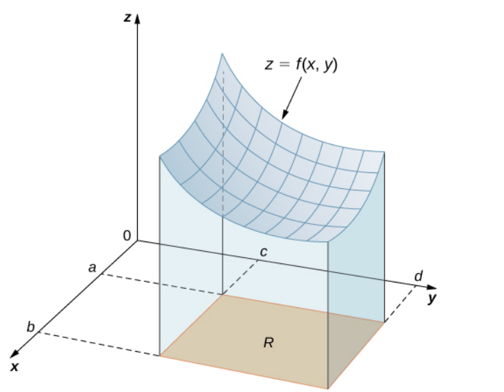
In this section, we will only consider rectangular reqions.

Note the similarity with of the idea with the "area under a curve" over an interval.

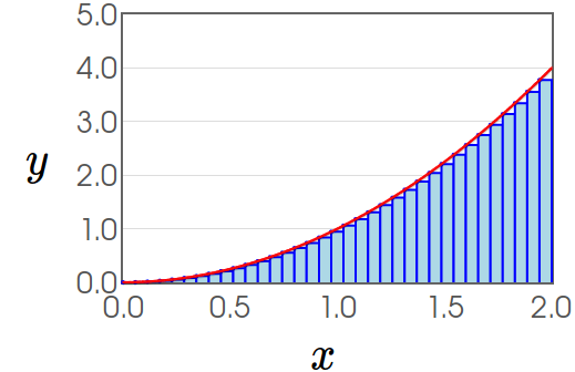
Recall: The Definite Integral

	$$\lim_{n \rightarrow \infty} \sum_{i=1}^{n} f(x_i^*)\,\Delta x$$
$\displaystyle \sum_{i=1}^{n} f(x_i^*)\,\Delta x$	$\longrightarrow$	$\displaystyle \int_{a}^{b} f(x) \,dx$
	$\longrightarrow$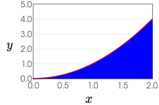

Double Integrals Over Rectangular Regions

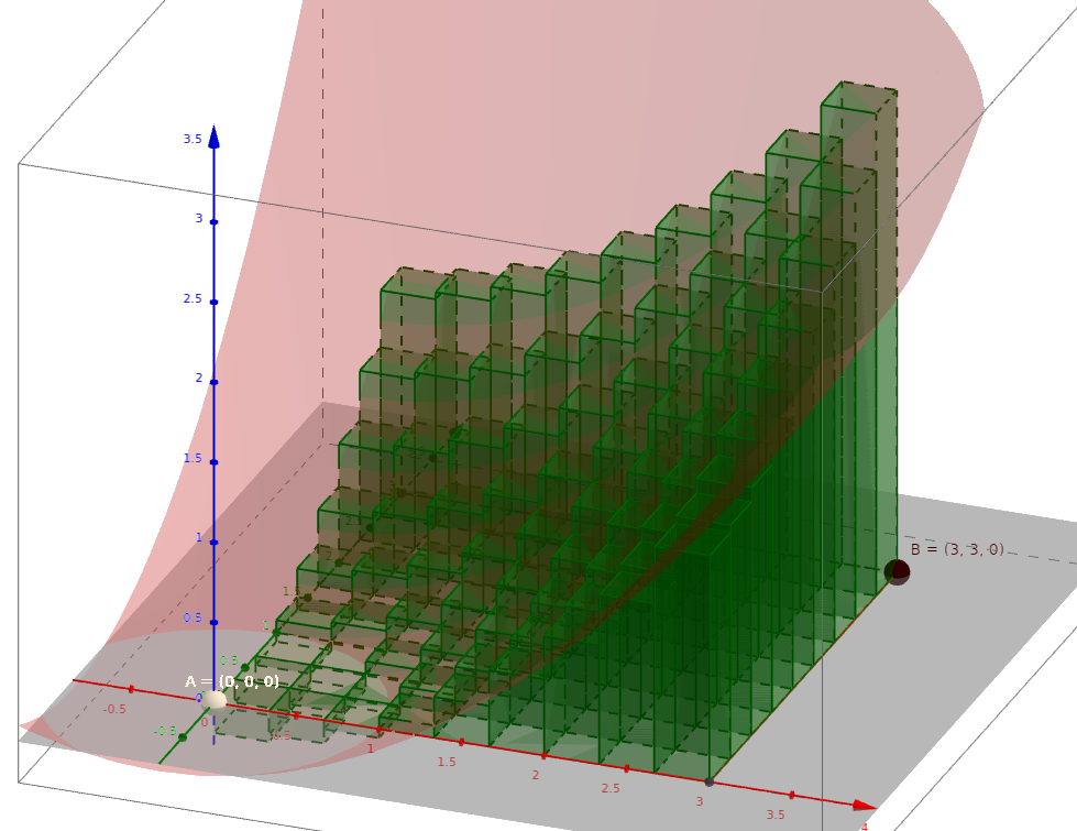
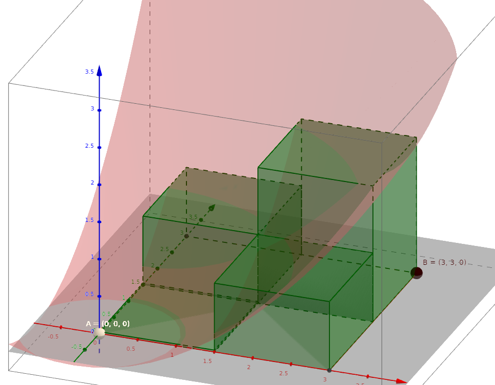
Just as we used rectangles to estimate the area under a curve, we estimate the volume under the surface over a rectangular region $R$ by using rectangular "boxes."

Double Integrals Over Rectangular Regions

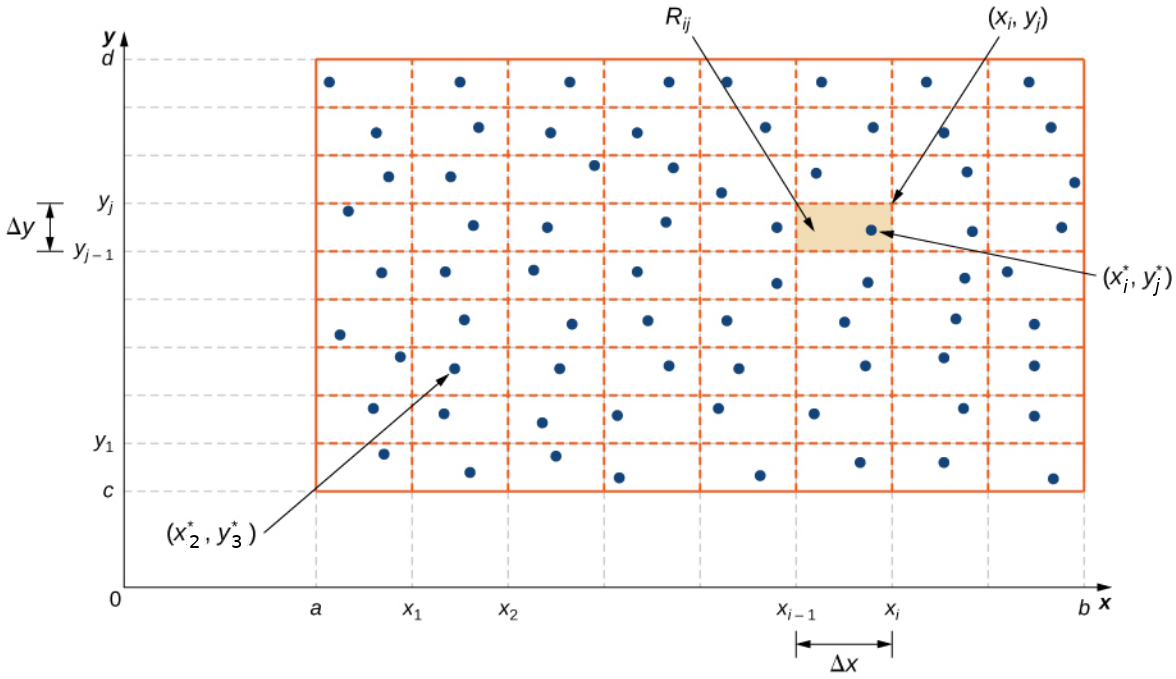
We construct our rectangular region $R$ as $[a,b]\times [c,d].$

Double Integrals Over Rectangular Regions

We then break up $[a,b]$ into $m$ intervals of size $\Delta x$ and $[c,d]$ into $n$ intervals of size $\Delta y.$

Note that $\displaystyle \Delta x=\frac{b-a}{m}$ and $\displaystyle \Delta y=\frac{d-c}{n}.$

Double Integrals Over Rectangular Regions

In each horizontal subinterval $[x_{i-1},x_{i}]$ we choose a point $x_i^*$ and in each vertical subinterval $[y_{j-1},y_{j}]$ we choose a point $y_j^*.$

Double Integrals Over Rectangular Regions

The height of the $ij$th rectangular box is $f(x_i^*,y_j^*)$ so that the volume of the $ij$th box is $$ f(x_i^*,y_j^*)\, \Delta x \, \Delta y=f(x_i^*,y_j^*)\, \Delta A $$

Double Integrals Over Rectangular Regions

Adding up all of volumes of all the boxes gives us an approximation of the volume under the surface. $$ \mbox{Volume}\approx\sum_{j=1}^{n}\sum_{i=1}^{m}f(x_i^*,y_j^*)\, \Delta A $$

Special Note

Just as areas under curves can be negative, so can volumes under surfaces.

When we compute volumes under surfaces, we call them "signed volumes."

Example

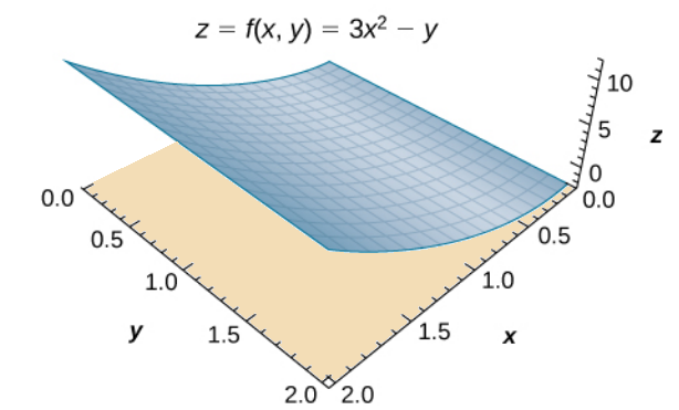
Approximate the double integral of the function $z = f (x, y) = 3x^2 - y$ over the rectangular region $R = [0, 2] \times [0, 2]$ by choosing $(x_i^*,y_j^*)$ to be: (a) the upper right corner of each sub-rectangle of $R,$ and (b) the midpoint of each sub-rectangle of $R.$

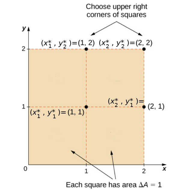
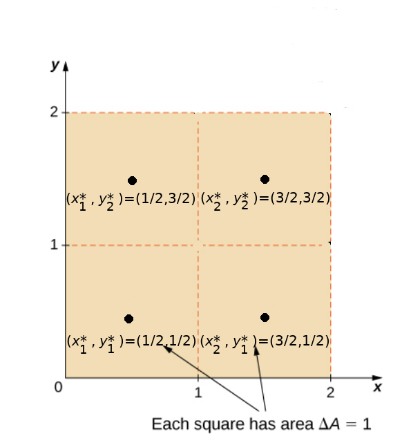
(a)The corner approximation is $$ \begin{array}{lll} \displaystyle \mbox{Volume} &\displaystyle\approx \sum_{j=1}^{2}\sum_{i=1}^{2}f(x_i^*,y_j^*)\, \Delta A&\mbox{}\\ \displaystyle &\displaystyle= f(x_1^*,y_1^*)\, \Delta A+f(x_2^*,y_1^*)\, \Delta A+f(x_1^*,y_2^*)\, \Delta A+f(x_2^*,y_2^*)\, \Delta A &\mbox{}\\ \displaystyle &\displaystyle= [f(x_1^*,y_1^*)+f(x_2^*,y_1^*)+f(x_1^*,y_2^*)+f(x_2^*,y_2^*)]\, \Delta A &\mbox{each rectangle has same area}\\ \displaystyle &\displaystyle= [f(1,1)+f(2,1)+f(1,2)+f(2,2)]\cdot 1 &\mbox{corner approx. with $\Delta A=1$}\\ \displaystyle &\displaystyle= 2+11+1+10&\mbox{}\\ \displaystyle &\displaystyle= 24&\mbox{}\\ \end{array} $$ The midpoint approximation is $$ \begin{array}{lll} \displaystyle \mbox{Volume} &\displaystyle\approx \sum_{j=1}^{2}\sum_{i=1}^{2}f(x_i^*,y_j^*)\, \Delta A &\mbox{}\\ \displaystyle &\displaystyle= f(x_1^*,y_1^*)\, \Delta A+f(x_2^*,y_1^*)\, \Delta A+f(x_1^*,y_2^*)\, \Delta A+f(x_2^*,y_2^*)\, \Delta A &\mbox{}\\ \displaystyle &\displaystyle= [f(x_1^*,y_1^*)+f(x_2^*,y_1^*)+f(x_1^*,y_2^*)+f(x_2^*,y_2^*)]\, \Delta A &\mbox{each rectangle has same area}\\ \displaystyle &\displaystyle= [f(0.5,0.5)+f(1.5,0.5)+f(0.5,1.5)+f(1.5,1.5)]\,\cdot 1 &\mbox{midpoint approx. with $\Delta A=1$}\\ \displaystyle &\displaystyle= 0.25+6.25+(-0.75)+5.25 &\mbox{}\\ \displaystyle &\displaystyle= 11 &\mbox{}\\ \end{array} $$

Double Integrals Over Rectangular Regions

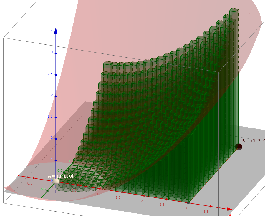
Of course, the more rectangular boxes we have, the better the approximation. $$ \mbox{Volume}\approx\sum_{j=1}^{n}\sum_{i=1}^{m}f(x_i^*,y_j^*)\, \Delta A $$

Double Integrals Over Rectangular Regions

	$\displaystyle \lim_{m,n \rightarrow \infty}\sum_{j=1}^{n}\sum_{i=1}^{m}f(x_i^,y_j^)\,\Delta A$
$\displaystyle \sum_{j=1}^{n}\sum_{i=1}^{m}f(x_i^,y_j^)\,\Delta A$	$\longrightarrow$	$\displaystyle \iint_{R} f(x,y) \,dA$
	$$\mbox{ }$$
	$\longrightarrow$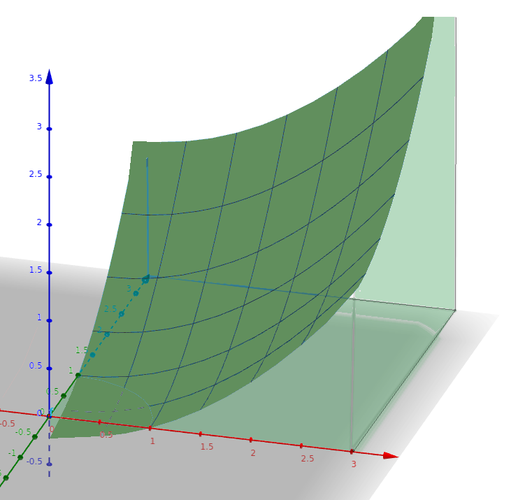

Double Integrals Over Rectangular Regions

The double integral of the function $f (x, y)$ over the rectangular region $R=[a,b]\times[c,d]$ in the $xy$-plane is defined as $$ \iint_{R} f(x,y) \,dA=\lim_{m,n \rightarrow \infty}\sum_{j=1}^{n}\sum_{i=1}^{m}f(x_i^*,y_j^*),\Delta A $$

When this limit exists, we say that $f(x,y)$ is integrable over $R.$

Properties of Double Integrals

Linearity Properties If $c$ is any constant, then $$ \begin{array}{ll} \displaystyle \iint_{R} f(x,y)+g(x,y) \,dA=\iint_{R} f(x,y) \,dA+\iint_{R} g(x,y) \,dA&\mbox{}\\ \displaystyle \iint_{R} cf(x,y)\,dA=c\iint_{R} f(x,y) \,dA&\mbox{}\\ \end{array} $$

Properties of Double Integrals

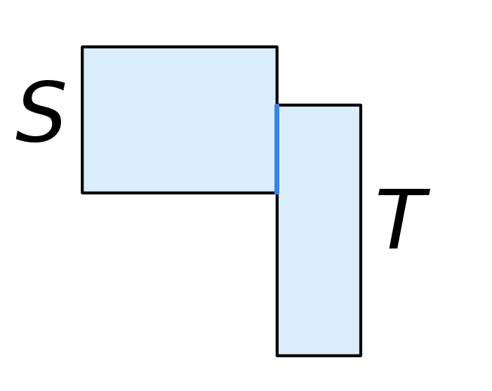
If $S$ and $T$ are two disjoint (non-overlapping) rectangular regions, that is $S \cap T=\varnothing,$ then $$ \begin{array}{ll} \displaystyle \iint_{S \cup T} f(x,y) \,dA=\iint_{S} f(x,y) \,dA+\iint_{T} f(x,y) \,dA&\mbox{}\\ \end{array} $$

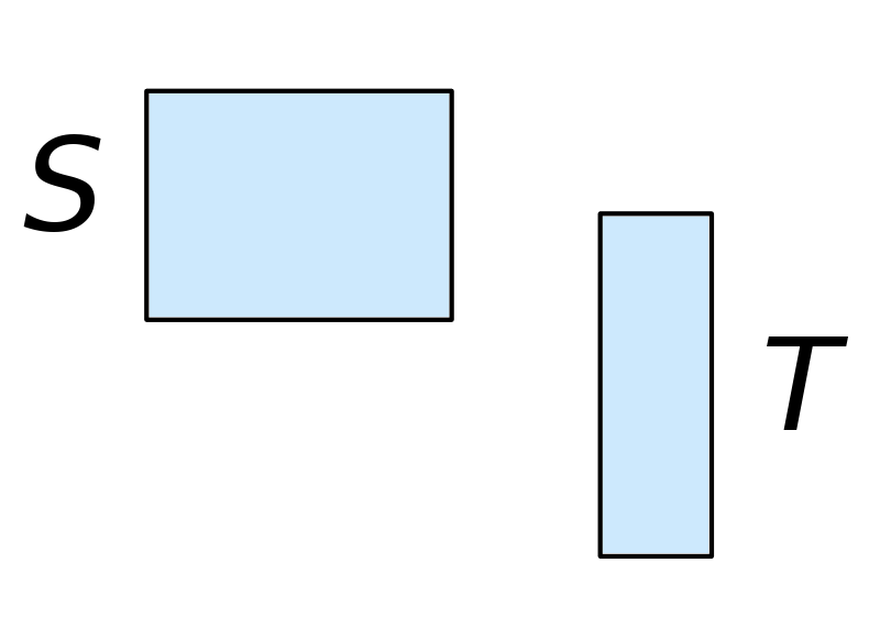
Special Note: The result $$\iint_{S \cup T} f(x,y) \,dA=\iint_{S} f(x,y) \,dA+\iint_{T} f(x,y) \,dA$$ still holds if the boundaries of $S$ and $T$ overlap.

Properties of Double Integrals

If $f(x,y)\geq g(x,y)$ on a region $R,$ then $$ \begin{array}{ll} \displaystyle \iint_{R} f(x,y) \,dA\geq \iint_{R} g(x,y) \,dA&\mbox{}\\ \end{array} $$

Properties of Double Integrals

Suppose $m$ and $M$ are real numbers and that $A(R)=(b-a)(d-c)$ is the area of the region $R.$ Then if $m \leq f (x, y) \leq M,$ $$ \begin{array}{ll} \ \displaystyle mA(R)\leq \iint_{R} f(x,y) \,dA\leq MA(R) \end{array} $$

Properties of Double Integrals

Assume that the functions $f (x, y)$ and $g(x, y)$ are integrable over the rectangular region $R$ and that $S$ and $T$ are subregions of $R.$ Also assume that $c,$ $m,$ and $M$ are real numbers. Then, $$ \begin{array}{ll} \displaystyle \iint_{R} f(x,y)+g(x,y) \,dA=\iint_{R} f(x,y) \,dA+\iint_{R} g(x,y) \,dA&\mbox{}\\ \displaystyle \iint_{R} cf(x,y)\,dA=c\iint_{R} f(x,y) \,dA&\mbox{}\\ \displaystyle S \cap T=\varnothing \implies \iint_{S \cup T} f(x,y) \,dA=\iint_{S} f(x,y) \,dA+\iint_{T} f(x,y) \,dA&\mbox{}\\ \displaystyle f(x,y)\geq g(x,y)\implies \iint_{R} f(x,y) \,dA\geq \iint_{R} g(x,y) \,dA&\mbox{}\\ \displaystyle m \leq f (x, y) \leq M\implies mA(R)\leq \iint_{R} f(x,y) \,dA\leq MA(R) \end{array} $$

Example

Consider the function $f(x,y)=27-2x^2-y^2$ over the region $R=[0,3]\times[0,3].$

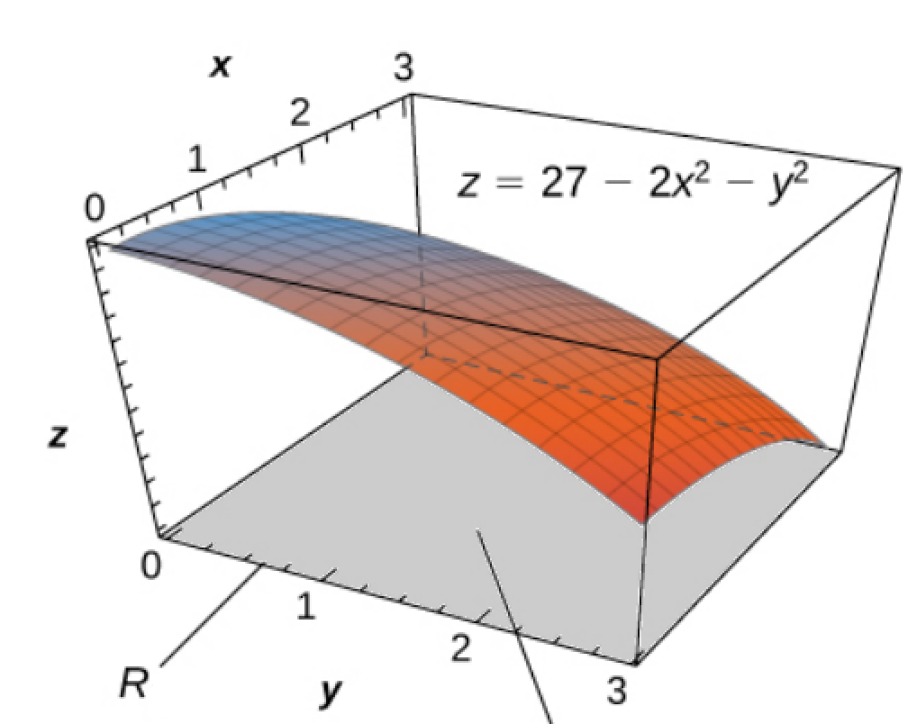
Give upper and lower bounds for the value of this integral.

We see that on the boundary of $R,$ the maximum value $M$ of $f(x,y)$ occurs at $(x,y)=(0,0),$ and the value is $$ M=f(0,0)=27. $$ We also see that on the boundary of $R,$ the minimum value $m$ of $f(x,y)$ occurs at $(x,y)=(3,3),$ and the value is $$ m=f(3,3)=0. $$ Using properties of integrals, we have $$ \begin{array}{lll} &\displaystyle 0=m \leq f (x, y) \leq M=27 &\mbox{}\\ \implies &\displaystyle mA(R)\leq \iint_{R} f(x,y) \,dA\leq MA(R)&\mbox{}\\ \implies &\displaystyle 0\cdot 9\leq \iint_{R} f(x,y) \,dA\leq 27 \cdot 9&\mbox{}\\ \implies &\displaystyle 0\leq \iint_{R} 27-2x^2-y^2 \,dA \leq 243&\mbox{}\\ \end{array} $$

Evaluating Double Integrals

We now begin learning the techniques for evaluating double integrals in a practical way.

Iterated Integrals

An iterated integral for a function $f (x, y)$ over the rectangular region $R = [a, b] \times [c, d]$ has one of two forms: $$ \int_{c}^{d}\int_{a}^{b} f(x,y) \,dx \,dy=\int_{c}^{d}\left[\int_{a}^{b} f(x,y) \,dx \right]\,dy $$ where $\displaystyle \int_{a}^{b} f(x,y) \,dx$ means we integrate with respect to $x$ while treating $y$ as a constant, or $$ \int_{a}^{b}\int_{c}^{d} f(x,y) \,dy \,dx=\int_{a}^{b}\left[\int_{c}^{d} f(x,y) \,dy \right]\,dx $$ where $\displaystyle \int_{c}^{d} f(x,y) \,dx$ means we integrate with respect to $y$ while treating $x$ as a constant.

Special Note

The integrals $\displaystyle \int_{a}^{b} f(x,y) \,dx$ and $\displaystyle \int_{c}^{d} f(x,y) \,dy$ are sometimes called partial integrals since we are integrating a multivariable function with respect to a single variable.

These partial integrals also have another interpretation:

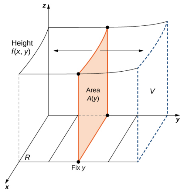
$\displaystyle \int_{a}^{b} f(x,y) \,dx$ defines a function of $y$ that gives the area under the surface $A(y)$ for a fixed value of $x.$

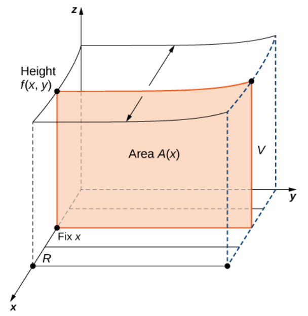
$\displaystyle \int_{c}^{d} f(x,y) \,dy$ defines a function of $x$ that gives the area under the surface $A(x)$ for a fixed value of $x.$

$\displaystyle A(y)=\int_{a}^{b} f(x,y) \,dx\,\,\,\,\,\,\,\,\,$	$\displaystyle A(x)=\int_{c}^{d} f(x,y) \,dy\,\,\,\,\,\,\,\,\,$

Fubini's Theorem

Fubini's Theorem nicely relates double integrals to iterated integrals.

Fubini's Theorem

Suppose that $f (x, y)$ is a function of two variables that is continuous over a rectangular region $R =\left\{(x, y) \in \mathbb{R}^2 |a \leq x \leq b, c \leq y \leq d \right\}.$ Then the double integral of $f(x,y)$ over the region equals the iterated integrals $$ \iint_{R} f(x,y)\,dA=\iint_{R} f(x,y)\,dx\, dy=\int_{c}^{d}\int_{a}^{b} f(x,y) \,dx \,dy $$ and $$ \iint_{R} f(x,y)\,dA=\iint_{R} f(x,y)\,dy\, dx=\int_{a}^{b}\int_{c}^{d} f(x,y) \,dy \,dx $$

Evaluating Double Integrals

$\displaystyle \iint_{R} f(x,y)\,dA=\int_{c}^{d}\color{#e86025}{\int_{a}^{b} f(x,y) \,dx} \,dy=\int_{c}^{d}A(y) \,dy\,\,\,\,\,\,\,\,\,$	$\displaystyle \iint_{R} f(x,y)\,dA =\int_{a}^{b}\color{#e86025}{\int_{c}^{d} f(x,y) \,dy} \,dx=\int_{a}^{b} A(x) \,dx\,\,\,\,\,\,\,\,\,$

We add up infinitely many "wafer-thin slices" of the solid in either the $y$ or $x$ direction to get the volume.

Evaluating Double Integrals

Using our properties of integrals together with Fubini's Theorem, we may now evaluate double integrals over rectangular regions in a practical way.

Example

Evaluate the double integral $$ \iint_R 3x^2 - y \, dA $$ over $R=[0,2]\times[0,2].$

Version #1: Integrate with respect to $x$ first. $$ \begin{array}{lll} \displaystyle \iint_R 3x^2 - y \, dA&\displaystyle= \int_{0}^{2}\int_{0}^{2} 3x^2 - y \,dx \, dy &\mbox{by The Great Fubini!}\\ \displaystyle &\displaystyle= \int_{0}^{2} \left[x^3 - yx\right]_{x=0}^{x=2} \, dy &\mbox{}\\ \displaystyle &\displaystyle= \int_{0}^{2} \left[2^3 - y\cdot 2\right]-\left[0^3 - y\cdot 0 \right] \, dy &\mbox{}\\ \displaystyle &\displaystyle= \int_{0}^{2} 8-2y \, dy &\mbox{}\\ \displaystyle &\displaystyle= \left[8y-y^2\right]_{0}^{2} &\mbox{}\\ \displaystyle &\displaystyle= \left[8\cdot 2-2^2\right]-\left[8\cdot 0-0^2\right] &\mbox{}\\ \displaystyle &\displaystyle= 12 &\mbox{}\\ \end{array} $$ Version #2: Integrate with respect to $y$ first. $$ \begin{array}{lll} \displaystyle \iint_R 3x^2 - y \, dA&\displaystyle= \int_{0}^{2}\int_{0}^{2} 3x^2 - y \,dy \, dx &\mbox{by The Great Fubini!}\\ \displaystyle &\displaystyle= \int_{0}^{2} \left[3x^2y-\frac{1}{2}y^2\right]_{y=0}^{y=2} \, dx &\mbox{}\\ \displaystyle &\displaystyle= \int_{0}^{2} \left[3x^2\cdot 2-\frac{1}{2}\cdot 2^2\right]-\left[3x^2\cdot 0-\frac{1}{2}\cdot 0^2\right] \, dx &\mbox{}\\ \displaystyle &\displaystyle= \int_{0}^{2} 6x^2-4 \, dx &\mbox{}\\ \displaystyle &\displaystyle= \left[2x^3-4x\right]_{0}^{2} &\mbox{}\\ \displaystyle &\displaystyle= \left[2\cdot 2^3-4\cdot 2\right]-\left[2\cdot 0^3-4\cdot 0\right] &\mbox{}\\ \displaystyle &\displaystyle= 12 &\mbox{}\\ \end{array} $$

The Order of Integration Sometimes Matters

Recall in second-term calculus that when we found special areas (i.e., areas between curves) and volumes (i.e., volumes of revolution) that sometimes it was much easier to integrate with respect to one variable than the other.

The same idea is true is true with double integrals.

Sometimes one order of integration is easier than another.

Example: Consider the double integral $$ \iint_R x\sin(xy) \,dA $$ over the region $R=[0,\pi]\times[1,2].$

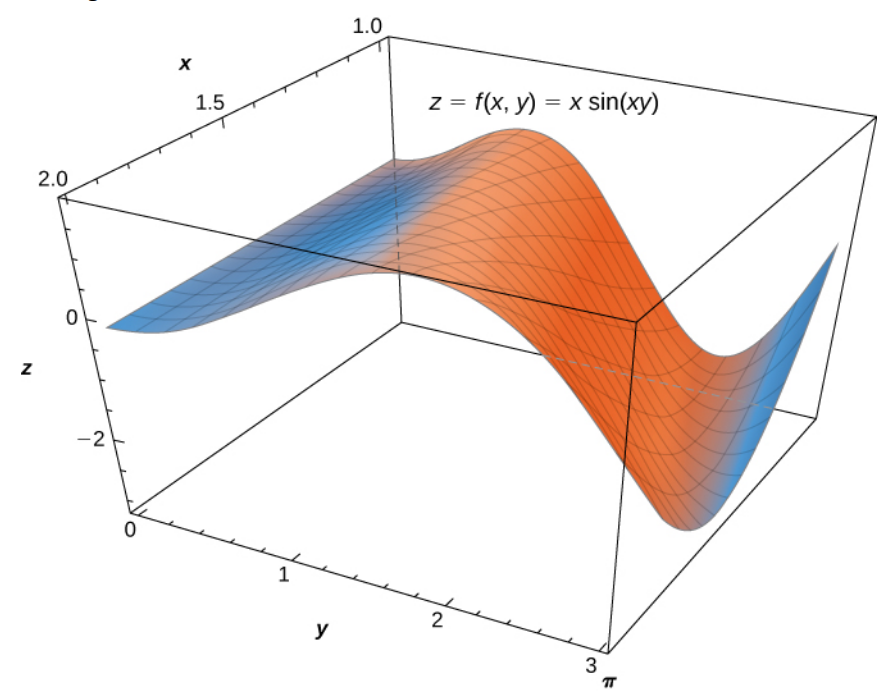
(a) Express the double integral in two different ways.

(b) Decide which double integral is easier to evaluate.

(c) Evaluate the integral.

(a) The Great Fubini tells us that $$ \begin{array}{lll} \displaystyle \iint_R x\sin(xy) \,dA&\displaystyle= \int_{1}^{2}\int_{0}^{\pi} x\sin(xy) \,dx \, dy&\mbox{Version 1}\\ \displaystyle &\displaystyle=\displaystyle \int_{0}^{\pi}\int_{1}^{2} x\sin(xy) \,dy \, dx &\mbox{Version 2}\\ \end{array} $$ (b) Version 1 (integrate w.r.t. $x$ first) would require integration by parts, whereas Version 2 (integrate w.r.t. $y$ first) treats the $x$ as a constant so that we can avoid integration by parts.

Thus, Version 2 is the easier integral.

(c) $$ \begin{array}{lll} \displaystyle \iint_R x\sin(xy) \,dA&\displaystyle= \int_{0}^{\pi}\int_{1}^{2} x\sin(xy) \,dy \, dx&\mbox{}\\ \displaystyle &\displaystyle=\displaystyle \int_{0}^{\pi} \left[-\cos(xy)\right]_{1}^{2} \, dx &\mbox{}\\ \displaystyle &\displaystyle=\displaystyle \int_{0}^{\pi} -\cos(2x)+\cos(x) \, dx &\mbox{}\\ \displaystyle &\displaystyle=\displaystyle \left[-\frac{1}{2}\sin(2x)+\sin(x)\right]_{0}^{\pi} &\mbox{}\\ \displaystyle &\displaystyle=\displaystyle \left[-\frac{1}{2}\sin(2\pi)+\sin(\pi)\right]-\left[-\frac{1}{2}\sin(2\cdot 0)+\sin(0)\right] &\mbox{}\\ \displaystyle &\displaystyle=\displaystyle 0 &\mbox{}\\ \end{array} $$

Volume of an Elliptic Paraboloid

Find the volume of the solid that is bounded by the elliptic paraboloid $2x^2 + y^2 + z = 27,$ the planes $x = 3,$ and $y = 3,$ and the three coordinate planes.

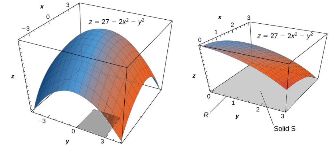
The volume of the solid is $$ \begin{array}{lll} \displaystyle \iint_R 27-2x^2-y^2 \,dA&\displaystyle=\int_{0}^{3}\int_{0}^{3} 27-2x^2-y^2 \, dy \, dx &\mbox{}\\ \displaystyle &\displaystyle=\int_{0}^{3} \left[27y-2x^2y-\frac{1}{3}y^3\right]_{0}^{3}\, dx &\mbox{}\\ \displaystyle &\displaystyle=\int_{0}^{3}\left[27\cdot 3-2x^2\cdot 3-\frac{1}{3}\cdot 3^3\right]-\left[27\cdot 0-2x^2\cdot 0-\frac{1}{3}\cdot 0^3\right]\, dx &\mbox{}\\ \displaystyle &\displaystyle=\int_{0}^{3}72-6x^2\, dx &\mbox{}\\ \displaystyle &\displaystyle=\left[72x-2x^3\right]_{0}^{3} &\mbox{}\\ \displaystyle &\displaystyle=\left[72\cdot 3-2\cdot 3^3\right]-\left[72\cdot 0-2\cdot 0^3\right] &\mbox{}\\ \displaystyle &\displaystyle=162 &\mbox{}\\ \end{array} $$

The Average Value of a Function $f(x,y)$ over a Region $R$

Recall that the average value of a single variable function $f(x)$ on an interval $[a,b]$ is defined to be $$ \displaystyle f_{avg}=\frac{1}{b-a}\int_{a}^{b} f(x)\, dx $$

The Average Value of a Function $f(x,y)$ over a Region $R$

The average value of a two-variable function $f(x,y)$ on a region $R$ is defined to be $$ \displaystyle f_{avg}=\frac{1}{A(R)}\iint_R f(x,y)\, dA $$

Example

Find the average value of the function $f(x,y)=27-2x^2-y^2$ over the region $R=[0,3]\times[0,3].$

$$ \begin{array}{lll} \displaystyle f_{avg}&\displaystyle= \frac{1}{A(R)}\iint_R f(x,y)\, dA&\mbox{}\\ \displaystyle &\displaystyle=\frac{1}{A(R)}\iint_R 27-2x^2-y^2\, dA &\mbox{}\\ \displaystyle &\displaystyle=\frac{1}{9}\cdot 162&\mbox{}\\ \displaystyle &\displaystyle=18&\mbox{}\\ \end{array} $$

Application

The weather map in the below shows an unusually moist storm system associated with the remnants of Hurricane Karl, which dumped $4$-$8$ inches ($100$-$200$ mm) of rain in some parts of the Midwest on September $22$-$23,$ $2010.$ The area of rainfall measured $300$ miles east to west and $250$ miles north to south.

Estimate the average rainfall over the entire area in those two days. Use a midpoint approximation of the double integral.

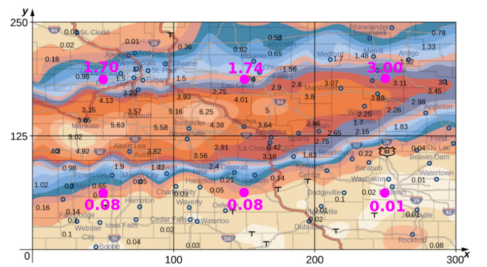
Let $f(x,y)$ be the rainfall function which gives the amount of rainfall at a point $(x,y)$ in the region $R=[0,300]\times[0,250]$ shown above.

The exact average can be expressed as $$ \displaystyle f_{avg}=\frac{1}{A(R)}\iint_R f(x,y)\, dA $$ However, we can only approximate this integral and will do so using the function values at the midpoints shown in the figure.

Now, using the figure we see that $\Delta x=100$ and $\Delta y=125.$

Thus, $\Delta A=\Delta x \Delta y=100 \cdot 125=12500.$

Then, using the values from the chart, $$ \begin{array}{lll} \displaystyle &\displaystyle\iint_R f(x,y)\, dA&\mbox{}\\ \displaystyle &\displaystyle\approx \sum_{j=1}^{2}\sum_{i=1}^{3} f(x_i^*,y_j^*)\Delta A&\mbox{}\\ \displaystyle &\displaystyle= f(x_1^*,y_1^*)\Delta A+f(x_2^*,y_1^*)\Delta A+f(x_3^*,y_1^*)\Delta A+f(x_1^*,y_2^*)\Delta A+f(x_2^*,y_2^*)\Delta A+f(x_3^*,y_2^*)\Delta A&\mbox{}\\ \displaystyle &\displaystyle= [f(x_1^*,y_1^*)+f(x_2^*,y_1^*)+f(x_3^*,y_1^*)+f(x_1^*,y_2^*)+f(x_2^*,y_2^*)+f(x_3^*,y_2^*)]\,\Delta A&\mbox{}\\ \displaystyle &\displaystyle= [f(50,62.5)+f(150,62.5)+f(250,62.5)+f(50,187.5)+f(150,187.5)+f(250,187.5)]\cdot 12500&\mbox{}\\ \displaystyle &\displaystyle= [0.08+0.08+0.01+1.70+1.74+3.00]\cdot 12500&\mbox{}\\ \displaystyle &\displaystyle= 82625&\mbox{}\\ \end{array} $$ Now, $A(R)=300\cdot 250=75000.$

From all of the above calculations, we conclude $$ \begin{array}{lll} \displaystyle f_{avg}&\displaystyle=\frac{1}{A(R)}\iint_R f(x,y)\, dA &\mbox{}\\ \displaystyle &\displaystyle\approx \frac{1}{75000}\cdot 82625 &\mbox{}\\ \displaystyle &\displaystyle\approx 1.10 &\mbox{}\\ \end{array} $$ That is, the average rainfall for the region was approximately $1.10$ inches of rain.