Tangent planes are a 3D analogue to tangent lines for single variable functions.
Tangent Planes
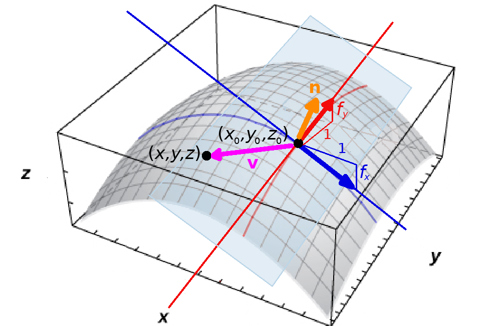
The tangent plane to a surface $S$ at the point $(x_0,y_0,z_0)$ is the plane made up of all possible tangent lines at $(x_0,y_0,z_0).$
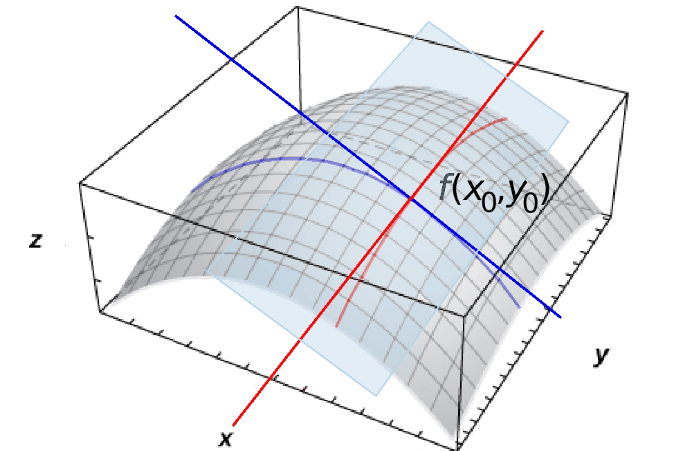
Tangent Planes
We shall now consider the problem of finding the tangent plane to a surface $z=f(x,y)$ at the point $(x_0,y_0,f(x_0,y_0)).$
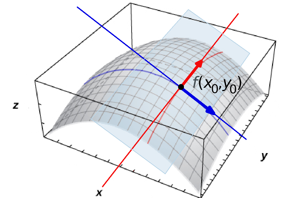
Tangent Planes
Consider the vectors in the tangent plane which extend one unit out in the positive $x$-direction and positive $y$-direction.

Tangent Planes
At the point $(x_0,y_0,f(x_0,y_0)),$ a tangent vector in the $x$-direction is ${\bf i}+f_x{\bf k}$ and in the $y$-direction is ${\bf j}+f_y{\bf k}$
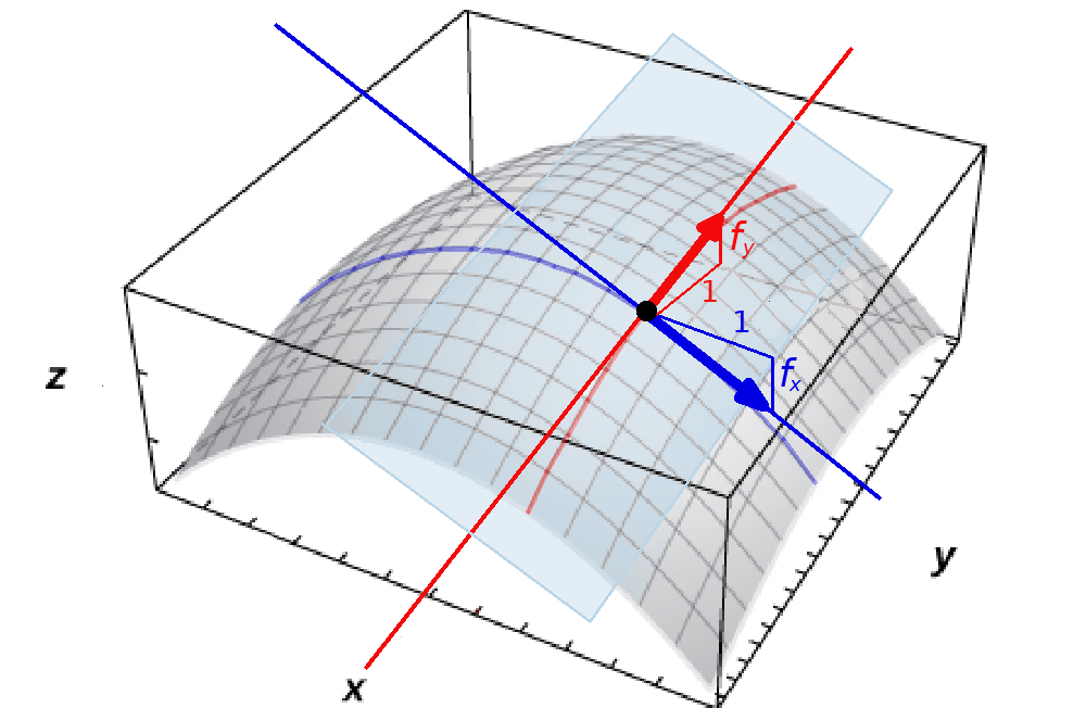
Tangent Planes
We may now find a normal vector ${\bf n}$ by computing the cross product of ${\bf i}+f_x{\bf k}$ and ${\bf j}+f_y{\bf k}$. That is,
${\bf n}$$=$$($${\bf i}+f_x{\bf k}$$)\times($${\bf j}+f_y{\bf k}$$)$
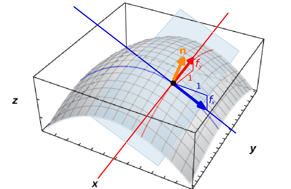
Tangent Planes
We now consider an arbitrary point in the tangent plane $(x,y,z).$ Then the vector ${\bf v}$ can be expressed in component form as $\langle x-x_0,y-y_0,z-z_0,\rangle.$ Since the normal vector ${\bf n}$ is orthogonal to the tangent plane, we know that
${\bf n}$ $\cdot$ ${\bf v}$$=0$
Tangent Planes
Using all of the above facts,
 $\color{darkorange}{{\bf n}}\cdot \color{magenta}{{\bf v}}=0$
$\implies [(\color{blue}{{\bf i}+f_x{\bf k}}$$)\times(\color{red}{{\bf j}+f_y{\bf k}})]\cdot\color{magenta}{\langle x-x_0,y-y_0,z-z_0,\rangle}$ $=0$
$\implies \color{darkorange}{\langle -f_x,-f_y,1\rangle}\cdot \color{magenta}{\langle x-x_0,y-y_0,z-z_0,\rangle}=0$
$$ -f_x\cdot(x-x_0)-f_y\cdot(y-y_0)+z-z_0=0 $$
Tangent Plane to a Surface $z=f(x,y)$
Let $S$ be a surface defined by a differentiable function $z = f (x, y),$ and let $(x_0, y_0)$ be a point in the domain of $f.$ Then, the equation of the tangent plane to $S$ at $(x_0, y_0)$ is given by $$ z=f(x_0,y_0)+f_x(x_0,y_0)(x-x_0)+f_y(x_0,y_0)(y-y_0) $$

Example
Find the equation of the tangent plane to the surface defined by the function $$f (x, y) = 2x^2 - 3xy + 8y^2 + 2x - 4y + 4$$ at point $(2, -1).$
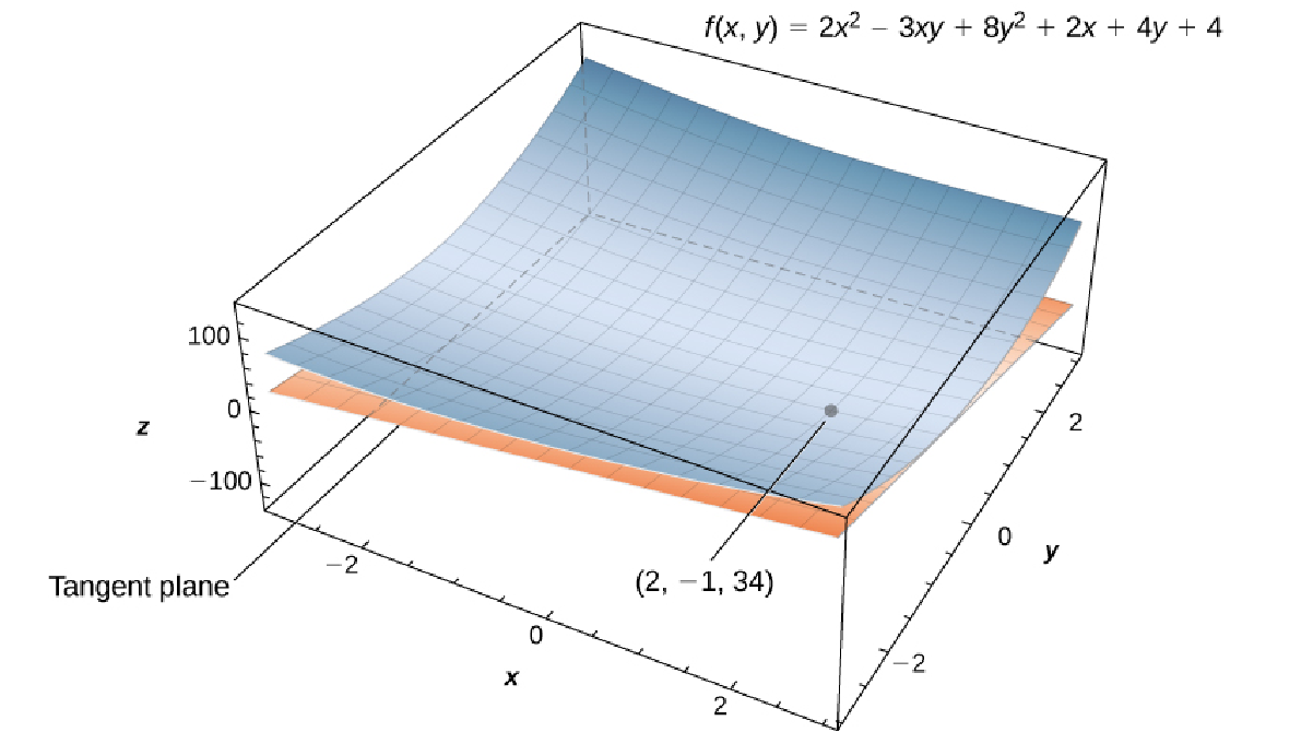
First we compute $f_x$ and $f_y.$
$$
f_x(x,y)=4x-3y+2,\,\,\,\,\,f_y(x,y)=-3x+16y-4
$$
Then,
$$
f_x(2,-1)=4(2)-3(-1)+2=13,\,\,\,\,\,f_y(x,y)=-3(2)+16(-1)-4=-26
$$
Second, we note that $$f(2,-1)=2(2)^2 - 3(2)(-1) + 8(-1)^2 + 2(2) - 4(-1) + 4=34.$$
Our tangent plane is then
$$
\begin{array}{lll}
\displaystyle z&\displaystyle= f(x_0,y_0)+f_x(x_0,y_0)(x-x_0)+f_y(x_0,y_0)(y-y_0)&\mbox{}\\
\displaystyle &\displaystyle= f(2,-1)+f_x(2,-1)(x-2)+f_y(2,-1)(y-(-1))&\mbox{}\\
\displaystyle &\displaystyle= 34+13(x-2)-26(y+1)&\mbox{}\\
\displaystyle &\displaystyle= 34+13x-26-26y-26&\mbox{}\\
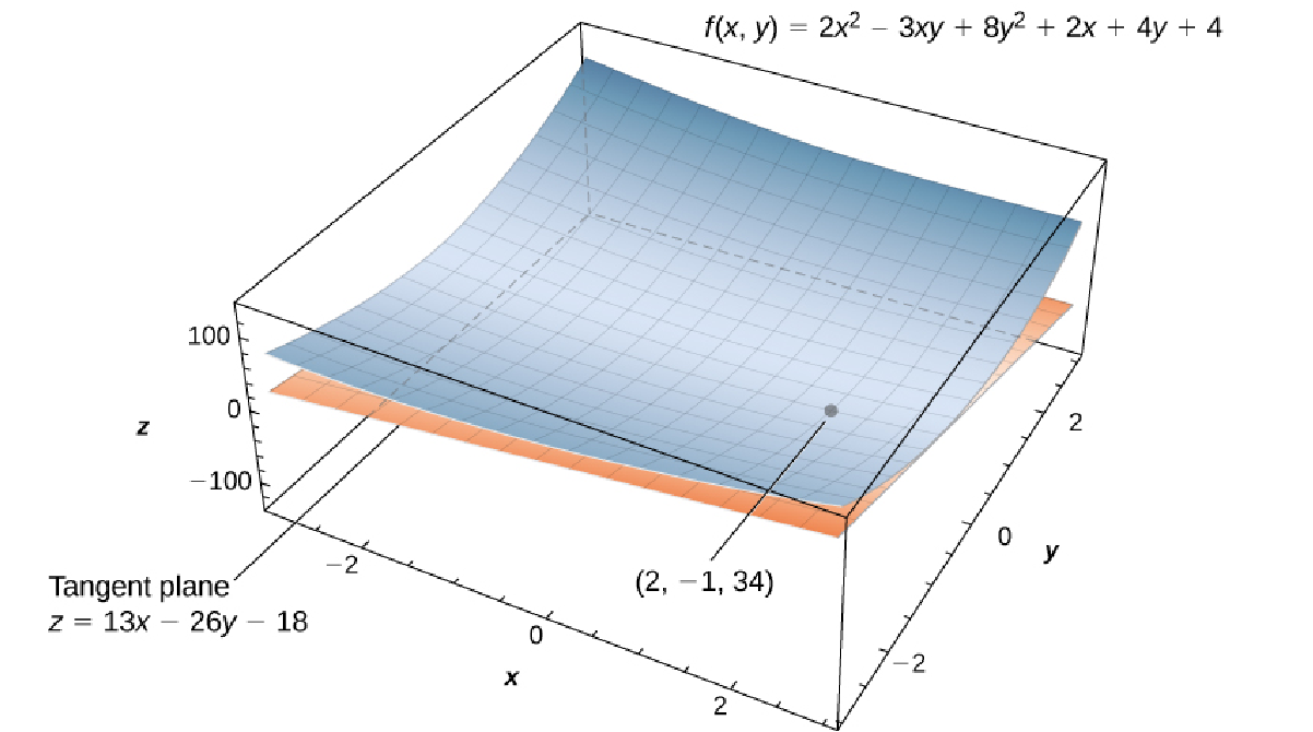
\displaystyle &\displaystyle= 13x-26y-18&\mbox{}\\
\end{array}
$$
Linear Approximations
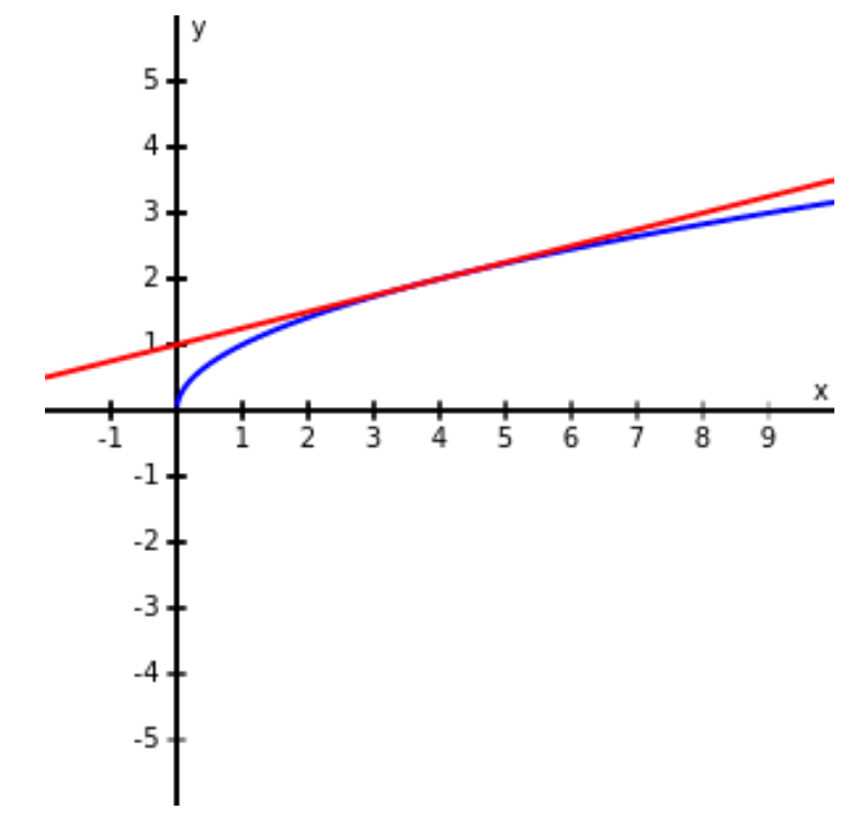
Recall the idea that a tangent line of a single variable function $y=f(x)$ at $x=a$ is a good approximation for $x$ near $a.$
Also recall that the tangent-approximation $L(x)=f'(a)(x-a)+f(a)$ is called the linearization of $f(x)$ at $a.$
Linear Approximations
Here we will extend that notion to functions of two variables...


Linear Approximations
Given a function $z = f (x, y)$ with continuous partial derivatives that exist at the point $(x_0, y_0),$ the linear approximation of $f(x,y)$ at the point $(x_0, y_0)$ is given by the equation $$L(x, y) = f (x_0, y_0) + f_x(x_0, y_0)(x - x_0) + f_y(x_0, y_0)(y - y_0)$$

Example
Given the function $$f (x, y) = 2x^2 - 3xy + 8y^2 + 2x - 4y + 4$$ use the linearization $L(x,y)=13x-26y-18$ at point $(2, -1)$ to approximate $f (2.1, -0.9.)$
$$
\begin{array}{lll}
\displaystyle f(2.1,-0.9)&\displaystyle\approx L(2.1,-0.9) &\mbox{}\\
\displaystyle &\displaystyle=13(2.1)-26(-0.9)-18 &\mbox{}\\
\displaystyle &\displaystyle=32.7 &\mbox{}\\
\end{array}
$$
The above value compares well to the exact value.
$$
f(2.1,-0.9)=2(2.1)^2 - 3(2.1)(-0.9) + 8(-0.9)^2 + 2(2.1) - 4(-0.9) + 4=32.77
$$
The advantage of using $L$ to approximate $f$ near $(2,-1)$ is that it is much easier to calculate. Plus, it still gives a reasonable approximation of $f.$
Example
Given the function $f (x, y) = e^{5 - 2x + 3y},$ find the linearization $L(x,y)$ at the point $(x_0,y_0)=(4, 1).$
Use the above to approximate the value of $f (4.1, 0.9).$
We first note that $f_x(x,y)=-2e^{5 - 2x + 3y}$ and $f_y(x,y)=3e^{5 - 2x + 3y}$ so that
$f_x(4,1)=-2$ and $f_y(4,1)=3.$
Then $$ \begin{array}{lll} \displaystyle L(x,y)&\displaystyle=f (x_0, y_0) + f_x(x_0, y_0)(x - x_0) + f_y(x_0, y_0)(y - y_0) &\mbox{}\\ \displaystyle &\displaystyle=f (4, 1) + f_x(4, 1)(x - 4) + f_y(4, 1)(y - 1) &\mbox{}\\ \displaystyle &\displaystyle=1-2(x - 4) + 3(y - 1) &\mbox{}\\ \displaystyle &\displaystyle=1-2x+8 + 3y - 3 &\mbox{}\\ \displaystyle &\displaystyle=-2x+ 3y+6 &\mbox{}\\ \end{array} $$ Thus, $$ f (4.1, 0.9)\approx L(4.1, 0.9)=-2\cdot 4.1+ 3\cdot 0.9+6=0.5 $$ For comparison, we note that $$ f(4.1,0.9)=0.6065306597... $$
Then $$ \begin{array}{lll} \displaystyle L(x,y)&\displaystyle=f (x_0, y_0) + f_x(x_0, y_0)(x - x_0) + f_y(x_0, y_0)(y - y_0) &\mbox{}\\ \displaystyle &\displaystyle=f (4, 1) + f_x(4, 1)(x - 4) + f_y(4, 1)(y - 1) &\mbox{}\\ \displaystyle &\displaystyle=1-2(x - 4) + 3(y - 1) &\mbox{}\\ \displaystyle &\displaystyle=1-2x+8 + 3y - 3 &\mbox{}\\ \displaystyle &\displaystyle=-2x+ 3y+6 &\mbox{}\\ \end{array} $$ Thus, $$ f (4.1, 0.9)\approx L(4.1, 0.9)=-2\cdot 4.1+ 3\cdot 0.9+6=0.5 $$ For comparison, we note that $$ f(4.1,0.9)=0.6065306597... $$
Differentiability
Recall the notion of differentiability of a single-variable function.
We have the very-cuddly definition that if the derivative exists at a point then function is said to be differentiable at that point.
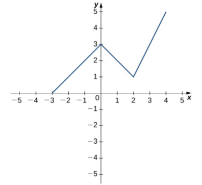
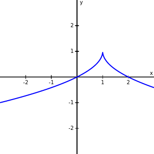
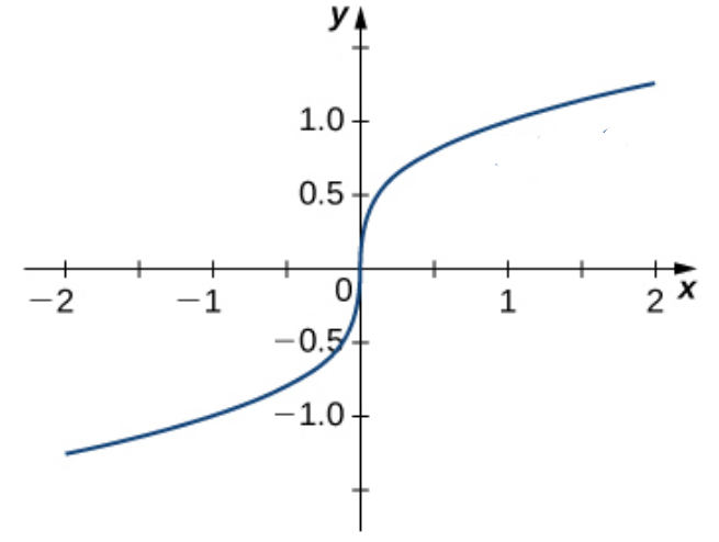
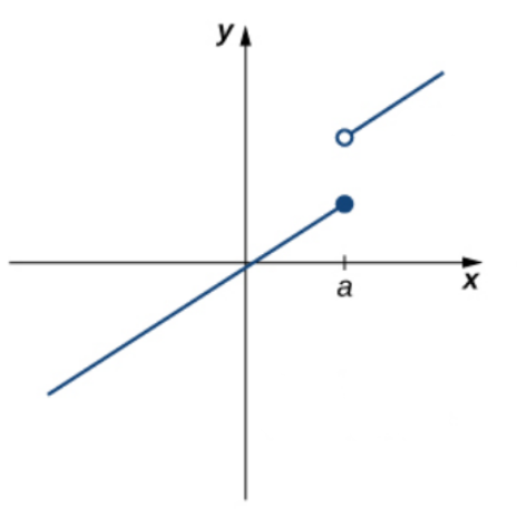
Sharp edges (corners and cusps), vertical tangent lines, and discontinuities are all places where differentiability can fail.
Differentiability
When we have two or more independent variables, the notion of differentiability at a point becomes more complicated since we can approach the point from any direction we like.
In the two-variable case, it would be great if differentiability at $(x_0,y_0)$ simply meant that $f_x$ and $f_y$ exist there, but it does not.
Multivariable differentiability is a bit more nuanced.
We shall presently use an example to illustrate the above point...
Example of a Non-Differentiable Function
Consider the function $$ f(x,y)= \begin{cases} \displaystyle \frac{xy}{\sqrt{x^2+y^2}} & \mbox{ if } (x,y)\neq (0,0)\\ \displaystyle 0 & \mbox{ if } (x,y)= (0,0) \end{cases} $$ $f_x(0,0)$ and $f_y(0,0)$ both exist, yet the tangent plane does not.
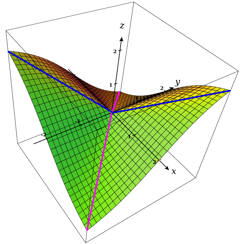
Definition of Differentiability
A function $f (x, y)$ is differentiable at a point $(x_0, y_0)$ if, for all points $(x, y)$ in a $\delta$ disk around $(x_0, y_0),$ we can write $$f (x, y) = f (x_0, y_0) + f_x (x_0, y_0)(x - x_0) + f_y (x_0, y_0)(y - y_0) + E(x, y),$$ where the error term $E$ satisfies $$ \lim_{(x,y)\rightarrow (x_0,y_0)} \frac{E(x,y)}{\sqrt{(x-x_0)^2+(y-y_0)^2}}=0 $$
Example
Use the definition of differentiability to show that $$ f(x,y)= \begin{cases} \displaystyle \frac{xy}{\sqrt{x^2+y^2}} & \mbox{ if } (x,y)\neq (0,0)\\ \displaystyle 0 & \mbox{ if } (x,y)= (0,0) \end{cases} $$ is not differentiable at $(0,0).$
Suppose that we can write $f(x,y)$ at $(0,0)$ as
$$
f (x, y) = f (0, 0) + f_x (0, 0)(x - 0) + f_y (0, 0)(y - 0) + E(x, y)=E(x,y)
$$
Then the error term is $f(x,y)$ itself. It follows that
$$
\begin{array}{lll}
\displaystyle \lim_{(x,y)\rightarrow (x_0,y_0)} \frac{E(x,y)}{\sqrt{(x-x_0)^2+(y-y_0)^2}}&\displaystyle=\lim_{(x,y)\rightarrow (0,0)} \frac{E(x,y)}{\sqrt{x^2+y^2}} &\mbox{}\\
\displaystyle &\displaystyle= \lim_{(x,y)\rightarrow (0,0)} \frac{\frac{xy}{\sqrt{x^2+y^2}}}{\sqrt{x^2+y^2}}&\mbox{}\\
\displaystyle &\displaystyle= \lim_{(x,y)\rightarrow (0,0)} \frac{xy}{x^2+y^2}&\mbox{}\\
\end{array}
$$
We claim that this limit does not exist.
To demonstrate this, suppose we approach $(0,0)$ along the $x$ axis. Then, the limit is $0$ since the expression $\displaystyle \frac{xy}{x^2+y^2}$ equals $0$ for all $x$ on the $x$-axis.
On the other hand, suppose that we approach $(0,0)$ along the line $y=x.$ Then $$\displaystyle \frac{xy}{x^2+y^2}=\frac{x\cdot x}{x^2+x^2}=\frac{x^2}{2x^2}=\frac{1}{2}$$ Thus, the limit is $\displaystyle \frac{1}{2}$ since the expression equals $\displaystyle \frac{1}{2}$ on the line $y=x$ (except at the origin).
Since the limit doesn't exist, the function $f(x,y)$ is not differentiable at $(0,0).$
Example
Use the definition of differentiability to show that $$ f(x,y)=2x^2-4y $$ is differentiable at $(2,-3).$
First, $f_x(x,y)=4x$ and $f_y(x,y)=-4$ so that $f_x(2,-3)=4\cdot 2=8$ and $f_y(2,-3)=-4.$
Also, $f(2,-3)=2(2)^2-4(-3)=8+12=20.$
Now, suppose that we can write $f(x,y)$ at $(2,-3)$ as $$ \begin{array}{lll} \displaystyle f(x,y)&\displaystyle= f (2,-3) + f_x (2,-3)(x - 2) + f_y (2,-3)(y - (-3)) + E(x, y)&\mbox{}\\ \displaystyle &\displaystyle= 20+8(x-2)-4(y+3)+E(x,y)&\mbox{}\\ \displaystyle &\displaystyle= 20+8x-16-4y-12+E(x,y)&\mbox{}\\ \displaystyle &\displaystyle= 8x-4y-8+E(x,y)&\mbox{}\\ \end{array} $$ Then the error term is $$E(x,y)=f(x,y)-(8x-4y-8)=2x^2-4y-8x+4y+8=2x^2-8x+8.$$ So, $$ \begin{array}{lll} \displaystyle \lim_{(x,y)\rightarrow (x_0,y_0)} \frac{E(x,y)}{\sqrt{(x-x_0)^2+(y-y_0)^2}}&\displaystyle=\lim_{(x,y)\rightarrow (2,-3)} \frac{2x^2-8x+8}{\sqrt{(x-2)^2+(y+3)^2}} &\mbox{}\\ \displaystyle &\displaystyle=\lim_{(x,y)\rightarrow (2,-3)} \frac{2x^2-8x+8}{\sqrt{(x-2)^2+(y+3)^2}} &\mbox{}\\ \displaystyle &\displaystyle=\lim_{(x,y)\rightarrow (2,-3)} \frac{2(x^2-4x+4)}{\sqrt{(x-2)^2+(y+3)^2}} &\mbox{}\\ \displaystyle &\displaystyle=\lim_{(x,y)\rightarrow (2,-3)} \frac{2(x-2)^2}{\sqrt{(x-2)^2+(y+3)^2}} &\mbox{}\\ \displaystyle &\displaystyle \leq \lim_{(x,y)\rightarrow (2,-3)} \frac{2\left[(x-2)^2+(y+3)^2\right]}{\sqrt{(x-2)^2+(y+3)^2}} &\mbox{}\\ \displaystyle &\displaystyle = \lim_{(x,y)\rightarrow (2,-3)} 2\sqrt{(x-2)^2+(y+3)^2} &\mbox{}\\ \displaystyle &\displaystyle = 2\cdot 0 &\mbox{}\\ \displaystyle &\displaystyle = 0 &\mbox{}\\ \end{array} $$ But, since $\displaystyle \frac{2x^2-8x+8}{\sqrt{(x-2)^2+(y+3)^2}}=\frac{2(x-2)^2}{\sqrt{(x-2)^2+(y+3)^2}}\geq 0$ for all $x$ and $y,$ it follows that $$ \lim_{(x,y)\rightarrow (x_0,y_0)} \frac{E(x,y)}{\sqrt{(x-x_0)^2+(y-y_0)^2}}=\lim_{(x,y)\rightarrow (2,-3)} \frac{2x^2-8x+8}{\sqrt{(x-2)^2+(y+3)^2}}\geq 0. $$ By the two inequalities above, and the Squeeze Theorem, it can only be that $$ \lim_{(x,y)\rightarrow (x_0,y_0)} \frac{E(x,y)}{\sqrt{(x-x_0)^2+(y-y_0)^2}}=\lim_{(x,y)\rightarrow (2,-3)} \frac{2x^2-8x+8}{\sqrt{(x-2)^2+(y+3)^2}}= 0. $$ Thus, $f(x,y)$ is differentiable at $(2,-3).$
Fact: The above definition is not easy to use.
However, the kinds of functions we will be dealing with in this course are well-behaved enough so that we may simply use the following result which is a bit more cuddly than the definition....
A Nice Result: Continuity of First Partials Implies Differentiability
Let $z = f (x, y)$ be a function of two variables with $(x_0, y_0)$ in the domain of $f.$
If $f (x, y),$ $f_x (x, y),$ and $f_y (x, y)$ all exist in a neighborhood of $(x_0, y_0)$ and are continuous at $(x_0, y_0),$ then $f (x, y)$ is differentiable there.
Special Note
For the function $$ f(x,y)= \begin{cases} \displaystyle \frac{xy}{\sqrt{x^2+y^2}} & \mbox{ if } (x,y)\neq (0,0)\\ \displaystyle 0 & \mbox{ if } (x,y)= (0,0) \end{cases} $$ it is true that $f_x(0,0)=0,$ but continuity fails since $$ \lim_{(x,y)\rightarrow (x,y)} f_x(x,y)\neq f_x(0,0) $$ since the limit doesn't exist.
Example
Use the above result to show that the function $f (x, y) = 2x^2 - 4y$ is differentiable at the point $(2, -3).$
We note that $f (x, y),$ $f_x (x, y),$ and $f_y (x, y)$ are defined everywhere and
are everywhere continuous,
Thus, they all exist in some neighborhood of $(2, -3)$ and are continuous at $(2, -3).$
By the above, we conclude that $f (x, y)$ is differentiable at $(2,-3).$
Thus, they all exist in some neighborhood of $(2, -3)$ and are continuous at $(2, -3).$
By the above, we conclude that $f (x, y)$ is differentiable at $(2,-3).$
Differentiability Implies Continuity
Let $z = f (x, y)$ be a function of two variables with $(x_0, y_0)$ in the domain of $f .$
If $f (x, y)$ is differentiable at $(x_0, y_0),$ then $f (x, y)$ is continuous at $(x_0, y_0).$
Recall Differentials
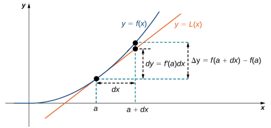
The differential of a function $y=f(x)$ is given by the equation $$dy=f'(x)dx.$$ The quantities $dy$ and $dx$ are called differentials.
The idea is that at any point along the curve, a "differential" (very small) change in $x,$ causes a "differential" change in $y.$
Recall Differentials
Differentials offer a nice way to approximate the change in a function. If we increase or decrease $x$ by a "differential" (small) amount $dx.$ This produces a small change in $y,$ say $\Delta y.$ To approximate this change at $x=a+dx$ we have $$\Delta y =f(a+dx)-f(a) \approx f'(a)(a+dx-a)=f'(a)dx=dy.$$ This is all to say that $$dy \approx \Delta y.$$

Differentials
We may extend the above idea to multivariable functions...
Differentials
If $f$ is differentiable at the point $(x_0, y_0),$ then the differentials $dx$ and $dy$ are defined as $dx = \Delta x$ and $dy = \Delta y.$
The differential $dz,$ called the total differential of $z = f (x, y)$ at $(x_0, y_0),$ is defined as $$dz = f_x (x_0, y_0)\,dx + f_y (x_0, y_0)\,dy.$$
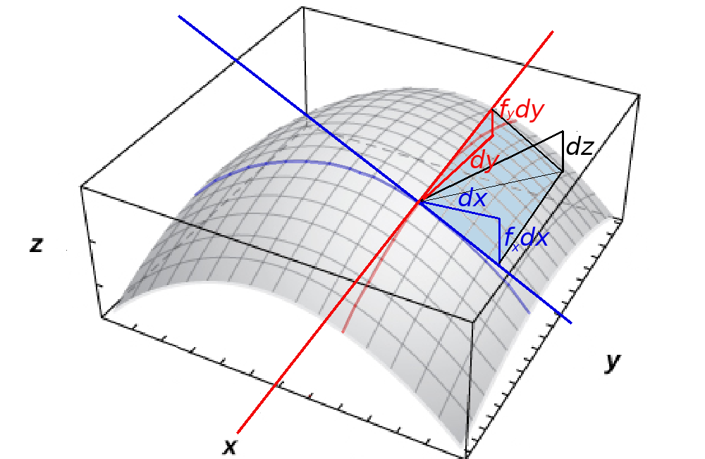
Differentials $$f(x_0+dx,y_0+dy) \approx f(x_0,y_0)+dz= f(x_0,y_0)+f_x (x_0, y_0)\,dx + f_y (x_0, y_0)\,dy.$$
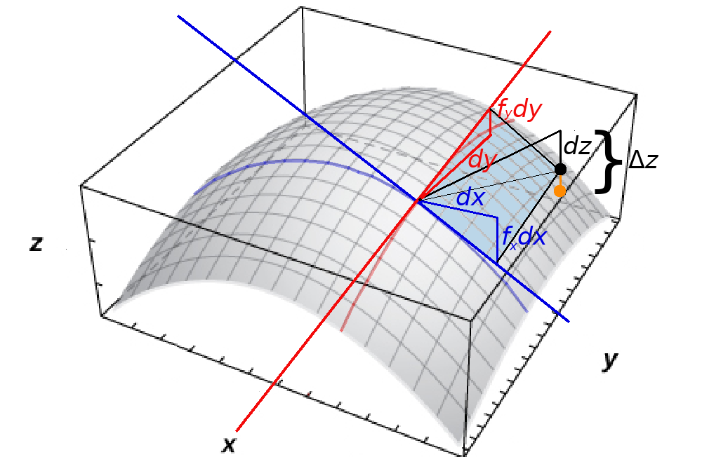
From the above we have that $\Delta z = f(x_0+dx,y_0+dy)-f(x_0,y_0) \approx dz.$
Example
Find the differential $dz$ of the function $f (x, y) = 4y^2 + x^2 y - 2xy$ and use it to approximate $\Delta z$ at point $(1, -1)$ using $dx = 0.03$ and $dy = -0.02.$
Find the exact value of $\Delta z.$
First, $f_x(x,y)=2xy-2y$ and $f_y(x,y)=8y+x^2-2x$ so that
$$f_x(1, -1)=2(1)(-1)-2(-1)=0$$ and $$f_y(1, -1)=8(-1)+(1)^2-2(1)=-9.$$
Then, $$ \begin{array}{lll} \displaystyle dz&\displaystyle= f_x(x,y)\,dx+f_y(x,y)\,dy&\mbox{}\\ \displaystyle &\displaystyle=f_x(1, -1)\,dx+f_y(1, -1)\,dy &\mbox{}\\ \displaystyle &\displaystyle=0\cdot 0.03+(-9)\,(-0.02) &\mbox{}\\ \displaystyle &\displaystyle=0.18 &\mbox{}\\ \end{array} $$ For comparison, $$ \begin{array}{lll} \displaystyle \Delta z&\displaystyle=f(x_0+dx,y_0+dy)-f(x_0,y_0) &\mbox{}\\ \displaystyle &\displaystyle=f(1+0.03,-1-0.02)-f(1,-1) &\mbox{}\\ \displaystyle &\displaystyle=f(1.03,-1.02)-f(1,-1) &\mbox{}\\ \displaystyle &\displaystyle=4(-1.02)^2 + 1.03^2 (-1.02) - 2(1.03)(-1.02)-(4(-1)^2 + 1^2 (-1) - 2(1)(-1)) &\mbox{}\\ \displaystyle &\displaystyle=0.180682 &\mbox{}\\ \displaystyle &\displaystyle\approx 0.18 &\mbox{}\\ \displaystyle &\displaystyle= dz &\mbox{}\\ \end{array} $$
Then, $$ \begin{array}{lll} \displaystyle dz&\displaystyle= f_x(x,y)\,dx+f_y(x,y)\,dy&\mbox{}\\ \displaystyle &\displaystyle=f_x(1, -1)\,dx+f_y(1, -1)\,dy &\mbox{}\\ \displaystyle &\displaystyle=0\cdot 0.03+(-9)\,(-0.02) &\mbox{}\\ \displaystyle &\displaystyle=0.18 &\mbox{}\\ \end{array} $$ For comparison, $$ \begin{array}{lll} \displaystyle \Delta z&\displaystyle=f(x_0+dx,y_0+dy)-f(x_0,y_0) &\mbox{}\\ \displaystyle &\displaystyle=f(1+0.03,-1-0.02)-f(1,-1) &\mbox{}\\ \displaystyle &\displaystyle=f(1.03,-1.02)-f(1,-1) &\mbox{}\\ \displaystyle &\displaystyle=4(-1.02)^2 + 1.03^2 (-1.02) - 2(1.03)(-1.02)-(4(-1)^2 + 1^2 (-1) - 2(1)(-1)) &\mbox{}\\ \displaystyle &\displaystyle=0.180682 &\mbox{}\\ \displaystyle &\displaystyle\approx 0.18 &\mbox{}\\ \displaystyle &\displaystyle= dz &\mbox{}\\ \end{array} $$
Measurement Error
In measurement there will always be some error. That is, we can never measure something like a length exactly.
Errors in one quantity causes errors in others. For example, an error in measuring the side length of a cube will cause error in the volume of that cube.
Here, when we measure some value of $x,$ we shall treat the error in our measurement as a small difference $dx$ from the desired quantity.
If some quantity $y$ depends on $x$ in some way, say $y=f(x),$ we can use differentials to approximate the error in $y,$ that is $\Delta y,$ with $dy.$
Error versus Relative Error
The relative error in a quantity $Q$ is the comparison of the change to the quantity $\Delta Q$ from some value $Q.$ That is, $$\mbox{Relative Error}=\frac{\Delta Q}{Q}.$$ When this value is expressed as a percentage, it is called the percent error and is computed as $$\mbox{Percent Error}=100 \cdot \frac{\Delta Q}{Q}.$$
Bonus Example
The apex of the Washington Monument is made of aluminum. At the time the monument was completed, it was $8.9$ inches ($23$ cm) tall with a base of $5.6$ inches ($14$ cm) square. It weighed $100$ ounces ($2.83$ kg).
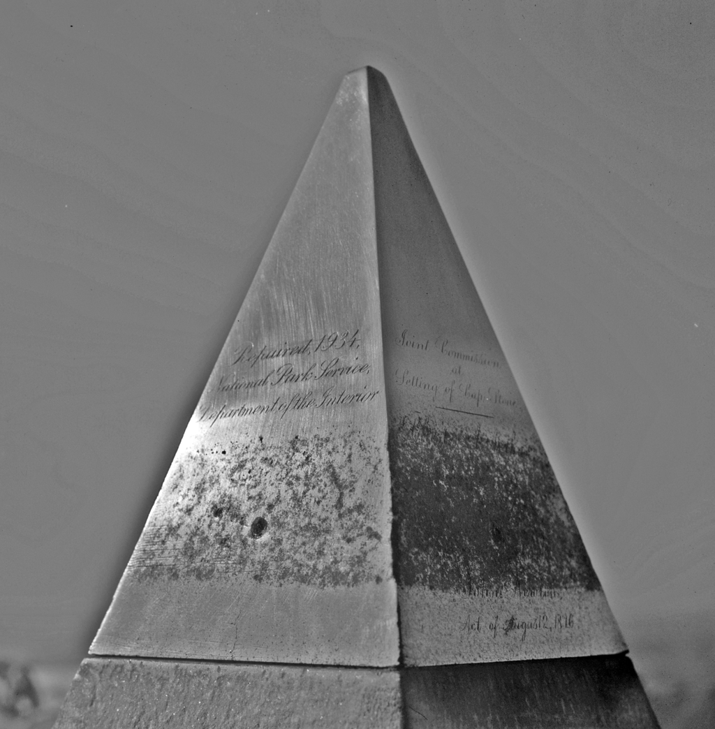
Suppose these measurements were made with an error of $\pm 0.2$ cm.
(a) Estimate the error in the computed volume of the apex.
(b) Estimate the relative error computed volume of the apex.
(c) Compute the exact error and the relative error in the area and compare to the estimate in part (a) and part (b).
(a) Let $b$ be the length of the base of a square pyramid and let $h$ be its height. The volume of the pyramid is then
$$
V(b,h)=\frac{1}{3}b^2h.
$$
It follows that
$$
dV=V_b(b,h)\,db+V_h(b,h)\,dh=\frac{2}{3}bh\,db+\frac{1}{3}b^2\,dh
$$
Since all measurements were made with an error of $\pm 0.2$ cm, we may say that $-0.2 \leq db \leq 0.2$ and $-0.2 \leq dh \leq 0.2.$
Then
$$
-0.2 \cdot \frac{2}{3}bh \leq \frac{2}{3}bh\,db \leq 0.2\cdot \frac{2}{3}bh
$$
and
$$
-0.2\cdot \frac{1}{3}b^2 \leq \frac{1}{3}b^2\,dh \leq 0.2 \cdot \frac{1}{3}b^2
$$
so that by adding the above two inequalities,
$$
-0.2 \cdot \frac{2}{3}bh-0.2\cdot \frac{1}{3}b^2 \leq dV \leq 0.2 \cdot \frac{2}{3}bh+0.2\cdot \frac{1}{3}b^2
$$
or
$$
-\frac{2}{15}bh- \frac{1}{15}b^2 \leq dV \leq \frac{2}{15}bh+\frac{1}{15}b^2
$$
For $b=14$ cm and $h=23$ cm, we have
$$
\begin{array}{lll}
&\displaystyle -\frac{2}{15}bh- \frac{1}{15}b^2 \leq dV \leq \frac{2}{15}bh+\frac{1}{15}b^2 &\mbox{}\\
\implies &\displaystyle -\frac{2}{15}(14)(23)- \frac{1}{15}14^2 \leq dV \leq \frac{2}{15}(14)(23)+\frac{1}{15}(14)^2 &\mbox{}\\
\implies &\displaystyle -56 \leq dV \leq 56 &\mbox{}\\
\end{array}
$$
Thus, the volume of the apex will be within $56$ cm3.
(b) The desired volume is $\displaystyle V(b,h)=\frac{1}{3}b^2h=\frac{1}{3}(14)^2 \cdot 23=\frac{4508}{3}=1502.\overline{6}$ cm3.
Thus, the relative error $\displaystyle \frac{\Delta V}{V}$ is approximately $$ -\frac{56}{1502.\overline{6}} =-\frac{6}{161}\leq \frac{dV}{V} \leq \frac{6}{161}=\frac{56}{1502.\overline{6}} $$ or $$ -0.03726708075... \leq \frac{dV}{V} \leq 0.03726708075... $$ Thus, the relative error in volume is about $3.7\%.$
(c) For $db=0.2$ and $dh=0.2,$ the exact error in volume is $$ \begin{array}{lll} \displaystyle \Delta V&\displaystyle= V(b+db,h+dh)-V(b,h)&\mbox{}\\ \displaystyle &\displaystyle=V(14+0.2,23+0.2)-V(14,23) &\mbox{}\\ \displaystyle &\displaystyle=V(14.2,23.2)-V(14,23) &\mbox{}\\ \displaystyle &\displaystyle=\frac{1}{3}(14.2)^2(23.2)-\frac{1}{3}14^2(23) &\mbox{}\\ \displaystyle &\displaystyle=56.682\overline{6} &\mbox{}\\ \end{array} $$ and for $db=-0.2$ and $dh=-0.2,$ $$ \begin{array}{lll} \displaystyle \Delta V&\displaystyle= V(b+db,h+dh)-V(b,h)&\mbox{}\\ \displaystyle &\displaystyle=V(14-0.2,23-0.2)-V(14,23) &\mbox{}\\ \displaystyle &\displaystyle=V(13.8,22.8)-V(14,23) &\mbox{}\\ \displaystyle &\displaystyle=\frac{1}{3}(13.8)^2(22.8)-\frac{1}{3}14^2(23) &\mbox{}\\ \displaystyle &\displaystyle=-55.322\overline{6}&\mbox{}\\ \end{array} $$ Thus, the exact error is $$ -55.322\overline{6}\leq \Delta V\leq 56.682\overline{6} $$ and the exact relative error is $$ \frac{-55.322\overline{6}}{1502.\overline{6}}\leq \frac{\Delta V}{V}\leq \frac{56.682\overline{6}}{1502.\overline{6}} $$ or $$ -0.03681632653\leq \frac{\Delta V}{V}\leq 0.03772138421... $$