A single-variable function maps a real number $x$ to a real number $f(x).$
A vector-valued function maps a real number $t$ to a vector in the plane ${\bf r}(t)=x(t)\,{\bf i}+y(t)\,{\bf j}$ or a vector in space ${\bf r}(t)=x(t)\,{\bf i}+y(t)\,{\bf j}+z(t)\,{\bf k}.$
Today, we get cozy with multivariable functions which map points in the plane $(x,y)$ to a number $f(x,y)$ or points in space $(x,y,z)$ to real numbers $f(x,y,z).$
In applications, multivariable are everywhere. For example, the temperature $T$ of a steel plate at a point $(x,y)$ at time $t$ can be described by a multivariable function $T(x,y,t).$
Functions of Two Variables
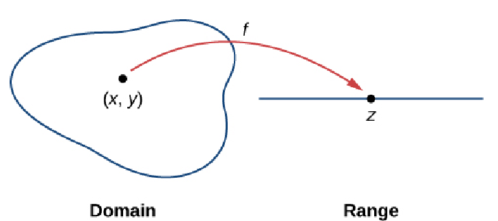
A function of two variables $z = f(x,y)$ maps each ordered pair $(x, y)$ in a subset $D$ of the real plane $\mathbb{R}^2$ to a unique real number $z.$
The set $D$ is called the domain of the function.
The range of $f$ is the set of all real numbers $z$ that has at least one ordered pair $(x, y)$ in $D$ such that $f (x, y)$ maps to $z.$
Example
Find the domain and range of the two-variable function $f (x, y) = \sqrt{9 - x^2 - y^2}.$
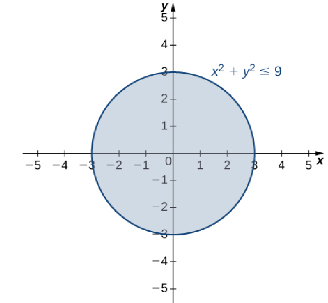
The expression under the square root, $9 - x^2 - y^2,$ must be non-negative so that $$ \begin{array}{lll} &\displaystyle 9 - x^2 - y^2 \geq 0&\mbox{}\\ \implies &\displaystyle x^2+y^2\leq 9&\mbox{}\\ \end{array} $$ Thus, the domain of $f$ is any $(x,y)$ whose distance from the origin is no greater than $3.$ More formally, $$ D=\{(x,y)\in\mathbb{R}^2|x^2+y^2\leq 9\} $$
We now find the range.
Since $\sqrt{9 - x^2 - y^2}$ is always greater than or equal to $0,$ we know $f(x,y)\geq 0$ for all ${(x,y)\in\mathbb{R}^2}.$
Also, the largest the expression $9 - x^2 - y^2$ can be is $9.$ Thus, the largest $f(x,y)$ can be is $3.$ Thus, $f(x,y)\leq 3$ for all ${(x,y)\in\mathbb{R}^2}.$
Thus, the range of $f$ is $ R=[0,3]. $
Other Examples
Find the domain and range of the two-variable function $g (x, y) = 3x + 5y + 2.$
$$D=\mathbb{R}^2, R=\mathbb{R}$$
Find the domain and range of the two-variable function $h (x, y) = x^2+y^2.$
$$D=\mathbb{R}^2, R=[0,\infty)$$
Graphing Functions of Two Variables
Just as a single variable function $f$ sends an $x$ on the real line to to a unique real number $f(x),$ a two-variable function $f$ sends an ordered pair $(x,y)$ in the plane to a unique real number $f(x,y).$
The points in space $(x,y,f(x,y))$ is the graph of $z=f(x,y).$
Such graphs are called surfaces.
Example
Graph the two-variable function $z=f (x, y) = \sqrt{9 - x^2 - y^2}.$
Squaring both sides of $z=f (x, y) = \sqrt{9 - x^2 - y^2}$ and rearranging, we have $x^2+y^2+z^2=9$
which we know to be a sphere of radius $3$ centered at the origin.
Since the range of $f$ is $[0,3]$ as shown earlier, we know the surface is the upper hemisphere of radius $3.$
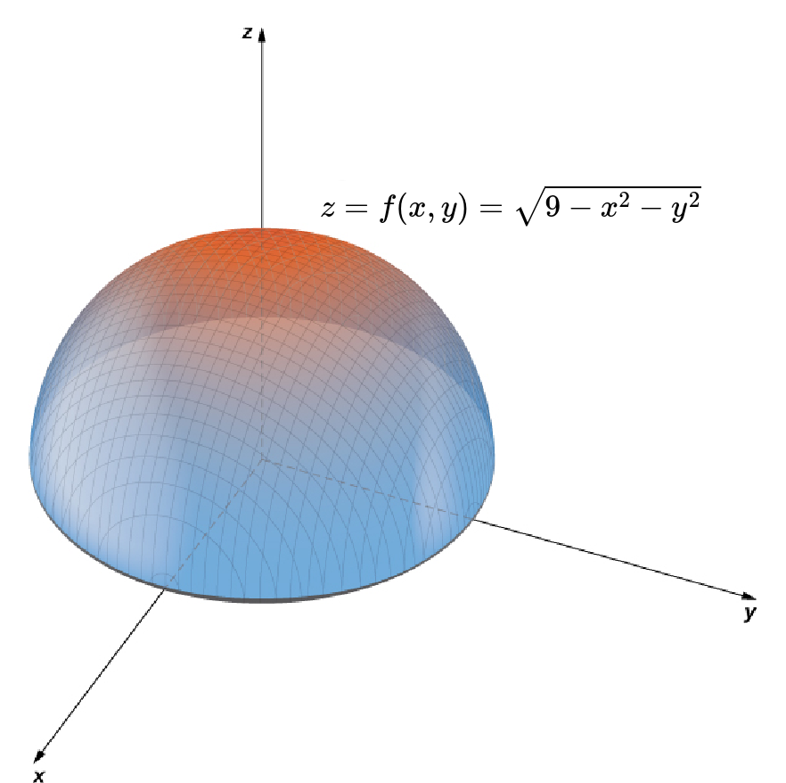
Since the range of $f$ is $[0,3]$ as shown earlier, we know the surface is the upper hemisphere of radius $3.$

Example
Graph the two-variable function $z=h (x, y) = x^2+y^2.$
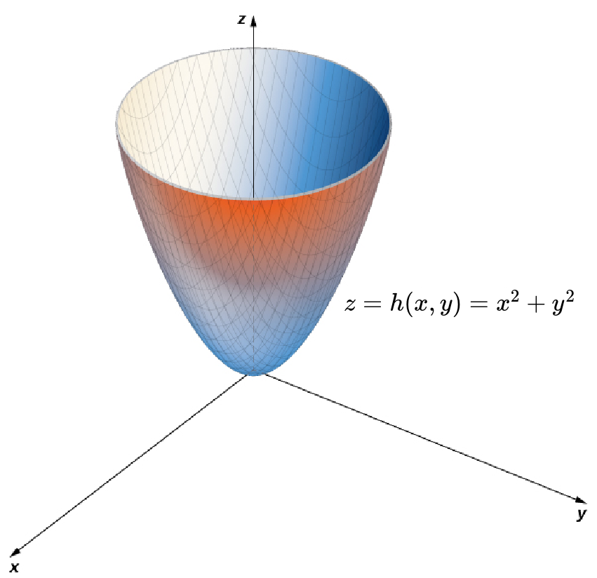
Setting $y=0,$ we see that the trace of the $xz$-plane is the equation $z=x^2.$
Similarly, setting $x=0,$ we see that the trace of the $yz$-plane is the equation $z=y^2.$
Taking horizontal slices (intersections with level planes), that is where $$h (x, y)=x^2+y^2=\mbox{constant},$$ we see that resulting curves are circles.
The surface is a paraboloid.
Similarly, setting $x=0,$ we see that the trace of the $yz$-plane is the equation $z=y^2.$
Taking horizontal slices (intersections with level planes), that is where $$h (x, y)=x^2+y^2=\mbox{constant},$$ we see that resulting curves are circles.
The surface is a paraboloid.

Level Curves
Topographical maps are two dimensional representations of three-dimensional land forms.
Points of equal elevation are plotted as curves.
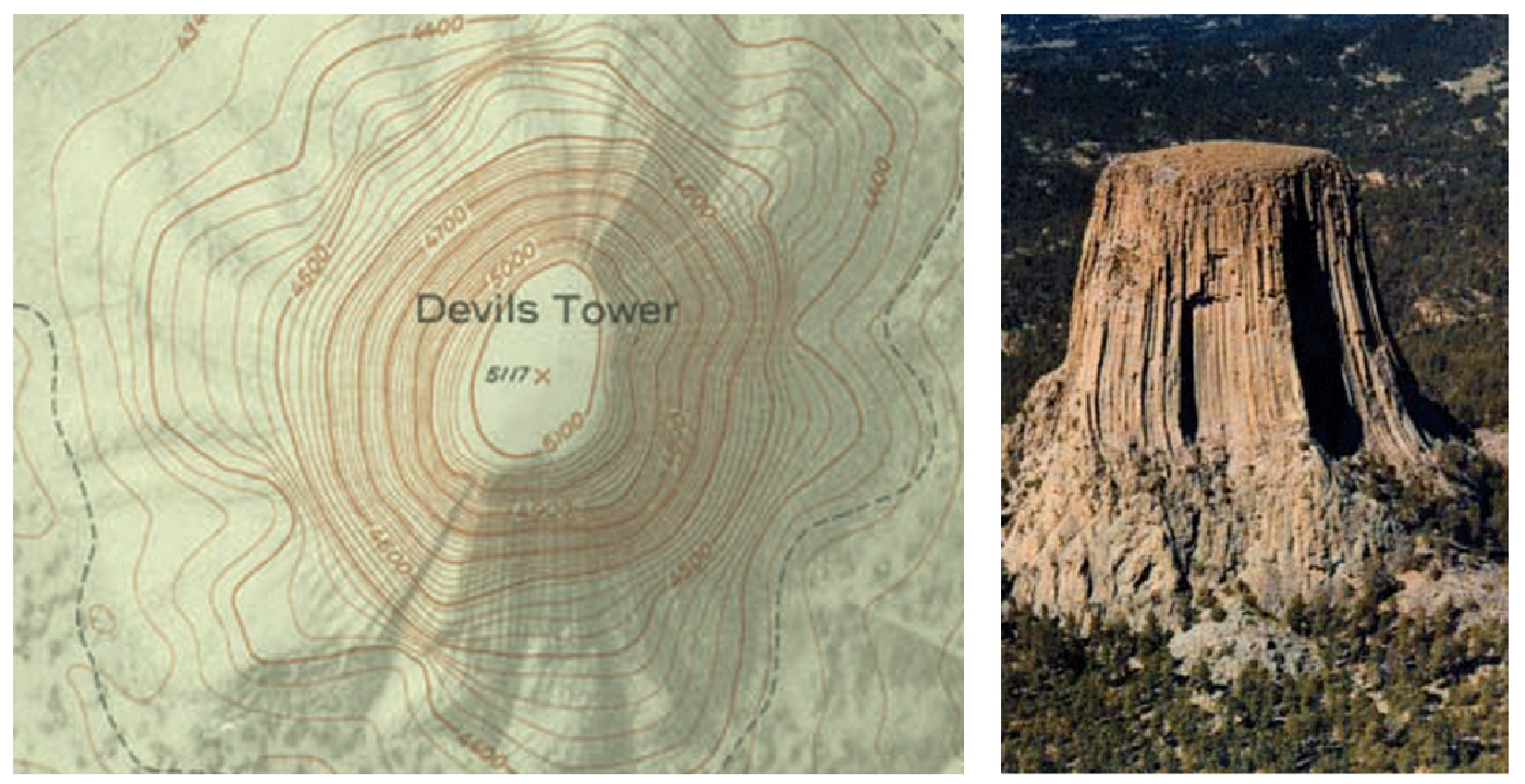
Notice that when the lines of the curves are closer together, the steeper the terrain.
Level Curves
Graphs of two-dimensional functions may also be understood using the same idea as a topographical map.
Points where the function values are equal are plotted as curves.
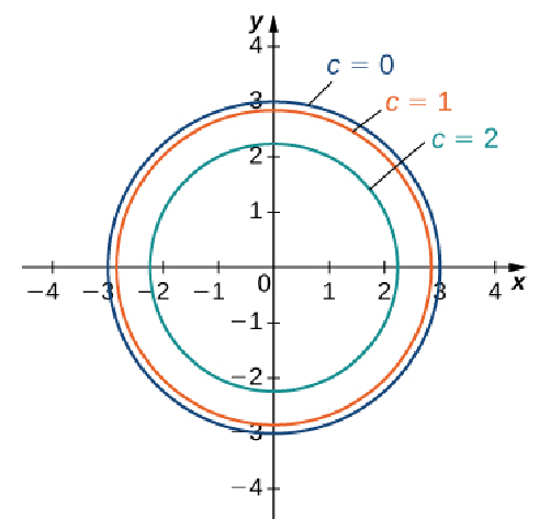

Above are the level curves $f(x,y)=0,$ $1,$ and $2.$
Level Curves
Given a function $f (x, y)$ and a number $c$ in the range of $f,$ a level curve of a function of two variables for the value $c$ is defined to be the set of points satisfying the equation $f (x, y) = c.$


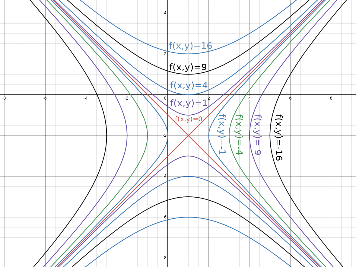
A graph of the various level curves of a function is called a contour diagram.
Example
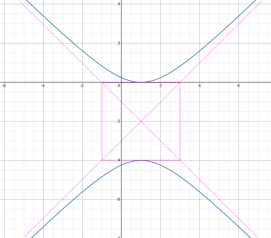
Given the function $f (x, y) = y^{2}-x^{2}+4y+2x+3,$ graph the level curve $f(x,y) = 4.$
The level curve $f(x,y) = 4$ gives the equation
$$
y^{2}-x^{2}+4y+2x+3=4
$$
Then
$$
\begin{array}{lll}
&\displaystyle y^{2}-x^{2}+4y+2x=1&\mbox{}\\
\implies &\displaystyle y^{2}+4y-x^{2}+2x=1&\mbox{}\\
\implies &\displaystyle y^{2}+4y-(x^{2}-2x)=1&\mbox{factor out minus}\\
\implies &\displaystyle y^{2}+4y\color{blue}{+4}\color{magenta}{-4}-(x^{2}-2x\color{blue}{+1}\color{magenta}{-1})=1&\mbox{}\\
\implies &\displaystyle (y+2)^2\color{magenta}{-4}-((x-1)^2\color{magenta}{-1})=1&\mbox{complete the square}\\
\implies &\displaystyle (y+2)^2-4-(x-1)^2+1=1&\mbox{redistribute minus}\\
\implies &\displaystyle (y+2)^2-(x-1)^2=4&\mbox{}\\
\implies &\displaystyle \frac{(y+2)^2}{2^2}-\frac{(x-1)^2}{2^2}=1&\mbox{}\\
\end{array}
$$
which is a vertically-aligned hyperbola shifted right by $1$ and down by $2.$

Example
Below is a contour diagram for $f (x, y) = y^{2}-x^{2}+4y+2x+3$ for $f(x,y)=0$, $\pm 1,$ $\pm 4,$ $\pm 9,$ and $\pm 16.$
Vertical Traces
While level curves are useful for understanding what a surface looks like, taking vertical slices of a surface can also reveal the nature of its shape.
Below, the vertical slices are parallel to the $xz$ and $yz$-planes.
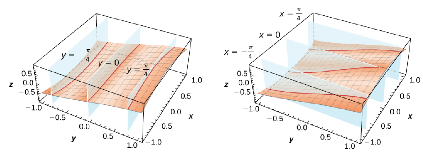
The resulting curves are called traces.
Vertical Traces
Consider a function $z = f (x, y)$ with domain $D \subseteq \mathbb{R}^2.$ A vertical trace of the function can be either the set of points that solves the equation $f (a, y) = z$ for a given constant $x = a$ or $f (x, b) = z$ for a given constant $y = b.$

Example
For the function $f(x,y)=\sin x\cos y,$ the vertical traces graphed below are
$\displaystyle z=f\left(x,-\frac{\pi}{4}\right),$ $\displaystyle z=f\left(x,0\right),$ and $\displaystyle z=f\left(x,\frac{\pi}{4}\right)$ for the graph on the left, and
$\displaystyle z=f\left(-\frac{\pi}{4},y\right),$ $\displaystyle z=f\left(0,y\right),$ and $\displaystyle z=f\left(\frac{\pi}{4},y\right)$ for the graph on the right.

Example
Given the function $f (x, y) = y^{2}-x^{2}+4y+2x+3,$ graph the vertical traces
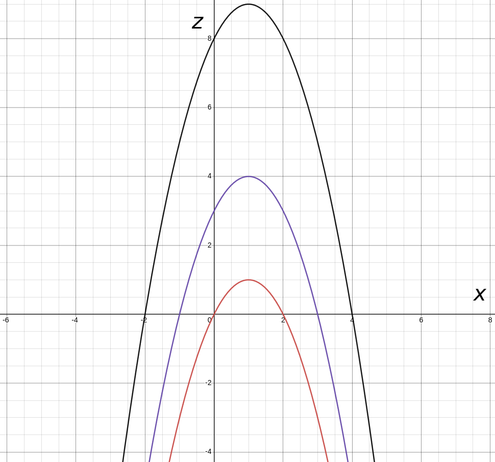
1) $z=f(x,-1),$ $z=f(x,0),$ and $z=f(x,1)$ in the $xz$-plane and
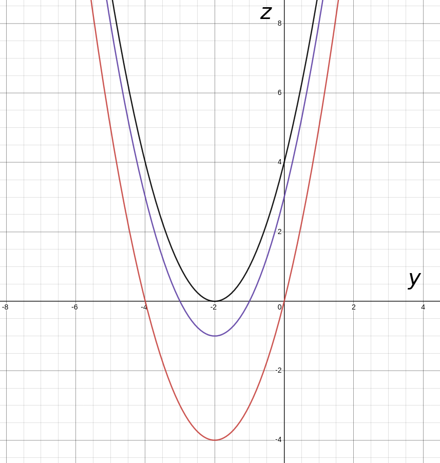
2) the vertical traces $z=f(-1,y),$ $z=f(0,y),$ and $z=f(1,y)$ in the $yz$-plane.
The vertical traces in the $xz$-plane:
$$
\color{#cc5652}{z=f(x,-1)=(-1)^{2}-x^{2}+4(-1)+2x+3=2x-x^2}\\
\color{#6f54ae}{z=f(x,0)=(0)^{2}-x^{2}+4(0)+2x+3=3+2x-x^2}\\
z=f(x,1)=(1)^{2}-x^{2}+4(1)+2x+3=8+2x-x^2
$$
The vertical traces in the $yz$-plane: $$ \color{#cc5652}{z=f(-1,y)=y^{2}-(-1)^{2}+4y+2(-1)+3=y^2+4y}\\ \color{#6f54ae}{z=f(0,y)=y^{2}-(0)^{2}+4y+2(0)+3=y^2+4y+3}\\ z=f(1,y)=y^{2}-(1)^{2}+4y+2(1)+3=y^2+4y+4\\ $$

The vertical traces in the $yz$-plane: $$ \color{#cc5652}{z=f(-1,y)=y^{2}-(-1)^{2}+4y+2(-1)+3=y^2+4y}\\ \color{#6f54ae}{z=f(0,y)=y^{2}-(0)^{2}+4y+2(0)+3=y^2+4y+3}\\ z=f(1,y)=y^{2}-(1)^{2}+4y+2(1)+3=y^2+4y+4\\ $$

Example
The level curves (contour diagram) and the vertical traces of $f (x, y) = y^{2}-x^{2}+4y+2x+3$ give us a good sense of what this surface looks like.


The $xz$ traces are downward-opening parabolas and the $xy$ traces are upward-opening parabolas.
The level curves are hyperbolas.
Example
The surface $f (x, y) = y^{2}-x^{2}+4y+2x+3$ is a hyperbolic paraboloid.
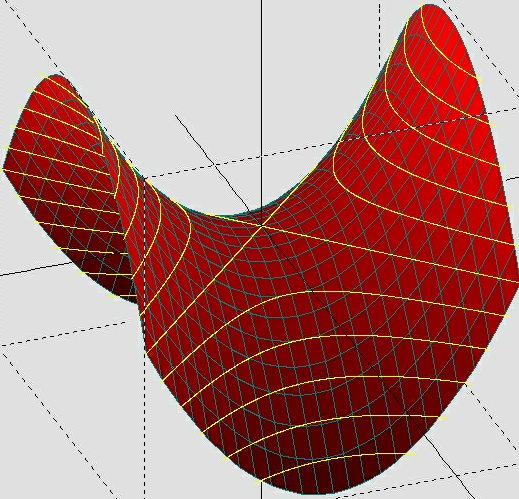
The $xz$ traces are downward-opening parabolas and the $yz$ traces are upward-opening parabolas.
The level curves are hyperbolas.
A surface may represent an object in-three dimensional space.
However, the variables need not be spatial dimensions.
Example
The temperature $u$ at a point $x$ on a thin, steel rod at time $t$ is modelled by a function $u (x, t).$

The $xu$ traces $u(x,c)$ are the temperature profiles of the rod at a particular time $c.$ For example, $u(x,0)$ is the initial temperature profile of the rod at time $0.$
Example
The temperature $u$ at a point $x$ on a thin, steel rod at time $t$ is modelled by a function $u (x, t).$
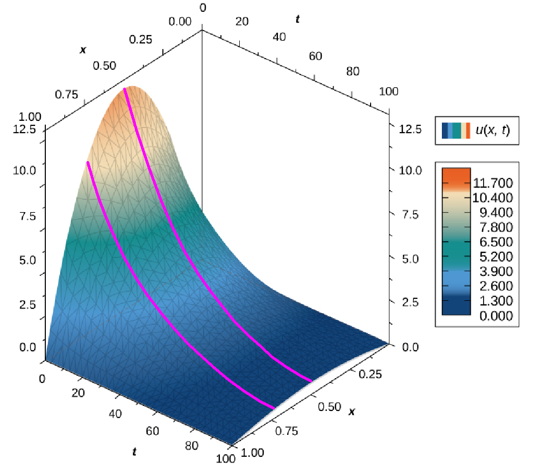
The $tu$ traces $u(c,t)$ give the temperature as a function of time at particular point $c$ on the rod.
Example
Suppose we need to model the steady-state temperature distribution in a thin plate made of iron located in the $xy$-plane.
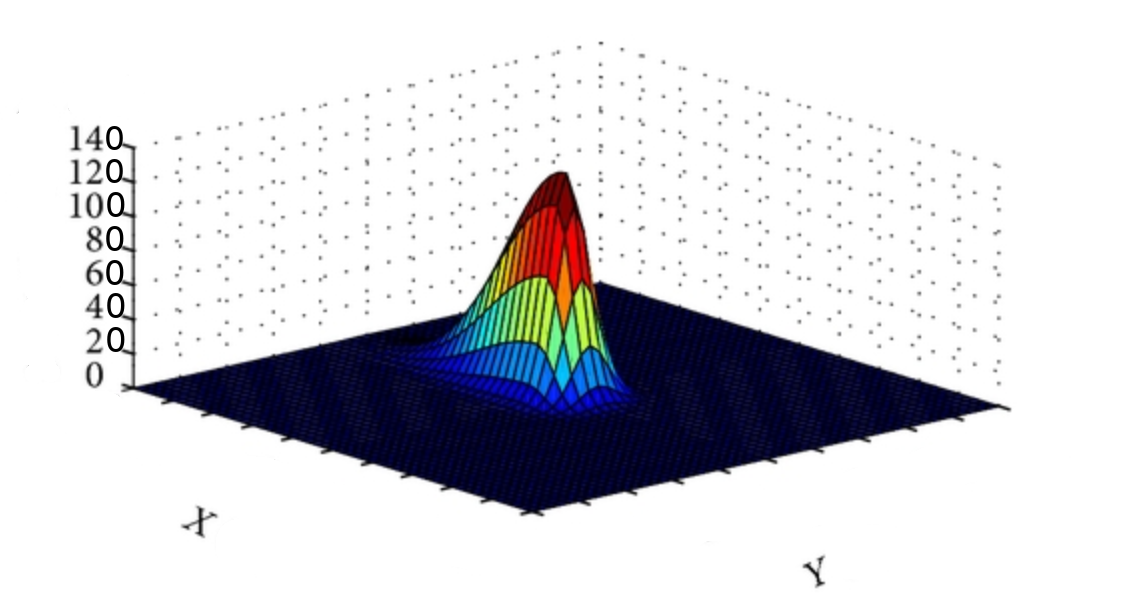
(a) Express $T$ as a function of $x$ and $y.$
(b) Determine the proportionality constant if the temperature at point $(0.1, -0.2)$ is $50^{\circ}\mbox{C}.$
(c) Find the level curve for $T (x,y)= 40^{\circ}\mbox{C}$ and describe what the curve represents.
(a) The square of the point $(x,y)$'s distance from the origin is $x^2+y^2.$ Thus, our function $T(x,y)$ has the form
$$
T(x,y)=\frac{k}{x^2+y^2+10}
$$
where $k$ is the proportionality constant.
(b) From the information given, $T(0.1, -0.2)=50.$ It follows that $$ \frac{k}{(0.1)^2+(-0.2)^2+10}=T(0.1, -0.2)=50 $$ so that $$ k=((0.1)^2+(-0.2)^2+10)\cdot 50=502.5 $$ Our function is then $$ T(x,y)=\frac{502.5}{x^2+y^2+10} $$ (c) We now find the level curve $T (x,y)= 40.$ This equation and the above equation give us $$ \frac{502.5}{x^2+y^2+10}=40 $$ which give $$ \frac{502.5}{10}=x^2+y^2+10\\ \implies 50.25-10=x^2+y^2\\ \implies x^2+y^2=40.25\\ \implies \sqrt{x^2+y^2}=\sqrt{40.25}\\ \implies \sqrt{x^2+y^2}\approx 6.34428877\\ $$ We interpret this to mean that the temperature is $40^{\circ}\mbox{C}$ at any point about $6.34$ centimeters from the origin.
(b) From the information given, $T(0.1, -0.2)=50.$ It follows that $$ \frac{k}{(0.1)^2+(-0.2)^2+10}=T(0.1, -0.2)=50 $$ so that $$ k=((0.1)^2+(-0.2)^2+10)\cdot 50=502.5 $$ Our function is then $$ T(x,y)=\frac{502.5}{x^2+y^2+10} $$ (c) We now find the level curve $T (x,y)= 40.$ This equation and the above equation give us $$ \frac{502.5}{x^2+y^2+10}=40 $$ which give $$ \frac{502.5}{10}=x^2+y^2+10\\ \implies 50.25-10=x^2+y^2\\ \implies x^2+y^2=40.25\\ \implies \sqrt{x^2+y^2}=\sqrt{40.25}\\ \implies \sqrt{x^2+y^2}\approx 6.34428877\\ $$ We interpret this to mean that the temperature is $40^{\circ}\mbox{C}$ at any point about $6.34$ centimeters from the origin.
Functions of Three Variables
Functions of three variables map a point in space $(x,y,z)$ to a real number $f(x,y,z).$
Although functions of three variables are different in many ways, the methods we've developed above for understanding functions of two variables carry over analogously.
Functions of Three Variables
Find the domain of the function $h(x, y, t) = (3t - 6)\sqrt{ y - 4x^2 + 4}.$
There are no restrictions on $t,$ but since $y - 4x^2 + 4$ is under a radical, we must impose the restriction that
$y - 4x^2 + 4\geq 0.$ Thus,
$$
D=\{(x,y,t)\in \mathbb{R}^3|y\geq 4x^2-4.\}
$$
Functions of Three Variables
Since the resulting graph $(x,y,z,f(x,y,z))$ is a four-dimensional object, we cannot visualize it directly.
However, we can begin to grasp the behavior of these functions by looking at "slices" just like we did for two dimensional surfaces.
Instead of looking at level curves $f(x,y)=c,$ we shall look at level surfaces $f(x,y,z)=c.$
Example
Find the level surface for the function $f (x, y, z) = 4x^2 + 9y^2 - z^2$ corresponding to $c = 1.$
The level surface corresponding to $c = 1$ is
$$
4x^2 + 9y^2 - z^2=1
$$
Then
$$
z^2=4x^2+9y^2-1
$$
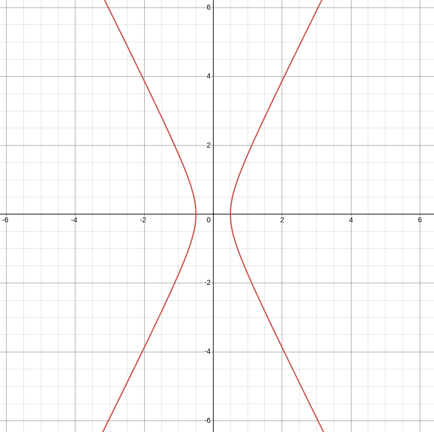
The vertical traces of this surface are $z^2=4x^2-1$ in the $xz$-plane
and $z^2=9y^2-1$ in the $yz$-plane.
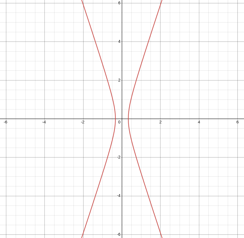
The level curves of our our level surface have the form $$ z^2=4x^2+9y^2-1=k $$ where $k$ is a constant. Thus, the level curves of this surface are ellipses.
From the above, the level surface corresponding to $c = 1$ is a hyperbola of one sheet.
Scenic Alternative
We could have simply recognized $4x^2 + 9y^2 - z^2=1$ as the equation of a quadric surface and put it into the form $\displaystyle \frac{x^2}{a^2}+\frac{y^2}{b^2}-\frac{z^2}{c^2}=1.$ That is, $$ \frac{x^2}{(1/2)^2}+\frac{y^2}{(1/3)^2}-\frac{z^2}{1^2}=1 $$ which we know to be a hyperboloid of one sheet.

and $z^2=9y^2-1$ in the $yz$-plane.

The level curves of our our level surface have the form $$ z^2=4x^2+9y^2-1=k $$ where $k$ is a constant. Thus, the level curves of this surface are ellipses.
From the above, the level surface corresponding to $c = 1$ is a hyperbola of one sheet.
Scenic Alternative
We could have simply recognized $4x^2 + 9y^2 - z^2=1$ as the equation of a quadric surface and put it into the form $\displaystyle \frac{x^2}{a^2}+\frac{y^2}{b^2}-\frac{z^2}{c^2}=1.$ That is, $$ \frac{x^2}{(1/2)^2}+\frac{y^2}{(1/3)^2}-\frac{z^2}{1^2}=1 $$ which we know to be a hyperboloid of one sheet.
Example
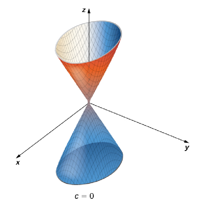
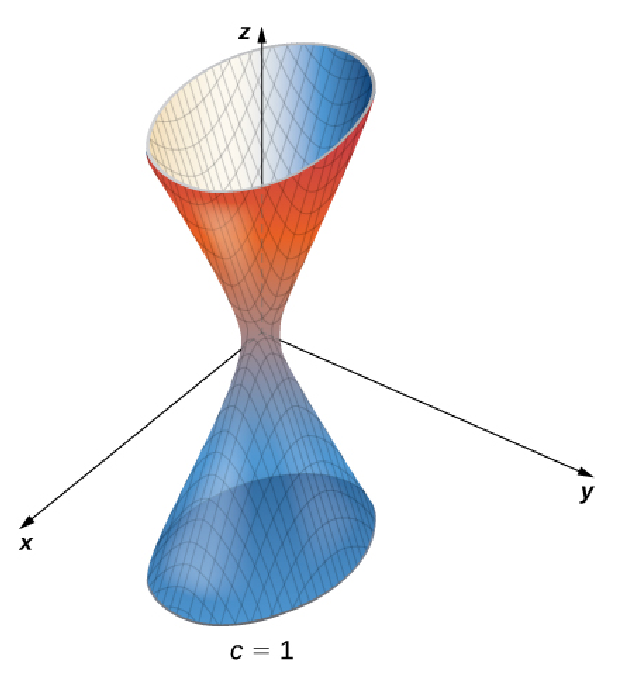
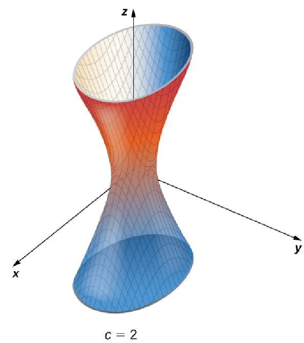
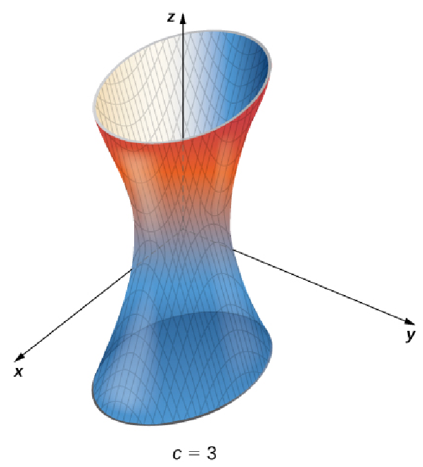
Below are some level surfaces for $f (x, y, z) = 4x^2 + 9y^2 - z^2=c$ for $c=0,$ $1,$ $2,$ and $3.$
Example
Suppose we need to model the steady-state temperature distribution in a block of iron located in $3$-dimensional space.
The temperature $T$ in degrees Celsius at a point $(x, y, z)$ is approximately inversely proportional to $10$ plus the square of its distance in centimeters from the origin.
(a) Express $T$ as a function of $x$ and $y$ and $z.$
(b) Determine the proportionality constant if the temperature at point $(0.1, -0.2, 0.1)$ is $50^{\circ}\mbox{C}.$
(c) Find the level surface for $T (x,y,z)= 40^{\circ}\mbox{C}$ and describe what it represents.
(a) The square of the point $(x,y,z)$'s distance from the origin is $x^2+y^2+z^2.$ Thus, our function $T(x,y,z)$ has the form
$$
T(x,y,z)=\frac{k}{x^2+y^2+z^2+10}
$$
where $k$ is the proportionality constant.
(b) From the information given, $T(0.1, -0.2,0,1)=50.$ It follows that $$ \frac{k}{(0.1)^2+(-0.2)^2+(0.1)^2+10}=T(0.1, -0.2,0.1)=50 $$ so that $$ k=((0.1)^2+(-0.2)^2+(0.1)^2+10)\cdot 50=503 $$ Our function is then $$ T(x,y,z)=\frac{503}{x^2+y^2+z^2+10} $$ (c) We now find the level curve $T (x,y,z)= 40.$ This equation and the above equation give us $$ \frac{503}{x^2+y^2+z^2+10}=40 $$ which give $$ \frac{503}{10}=x^2+y^2+z^2+10\\ \implies 50.3-10=x^2+y^2+z^2\\ \implies x^2+y^2+z^2=40.3\\ \implies \sqrt{x^2+y^2+z^2}=\sqrt{40.3}\\ \implies \sqrt{x^2+y^2+z^2}\approx 6.348228099\\ $$ We interpret this to mean that the temperature is $40^{\circ}\mbox{C}$ at any point about $6.34$ centimeters from the origin.
(b) From the information given, $T(0.1, -0.2,0,1)=50.$ It follows that $$ \frac{k}{(0.1)^2+(-0.2)^2+(0.1)^2+10}=T(0.1, -0.2,0.1)=50 $$ so that $$ k=((0.1)^2+(-0.2)^2+(0.1)^2+10)\cdot 50=503 $$ Our function is then $$ T(x,y,z)=\frac{503}{x^2+y^2+z^2+10} $$ (c) We now find the level curve $T (x,y,z)= 40.$ This equation and the above equation give us $$ \frac{503}{x^2+y^2+z^2+10}=40 $$ which give $$ \frac{503}{10}=x^2+y^2+z^2+10\\ \implies 50.3-10=x^2+y^2+z^2\\ \implies x^2+y^2+z^2=40.3\\ \implies \sqrt{x^2+y^2+z^2}=\sqrt{40.3}\\ \implies \sqrt{x^2+y^2+z^2}\approx 6.348228099\\ $$ We interpret this to mean that the temperature is $40^{\circ}\mbox{C}$ at any point about $6.34$ centimeters from the origin.