Today, we begin the process of finding areas under curves.
As we shall see through out the course, there are many applications which reduce to finding the area under a curve.
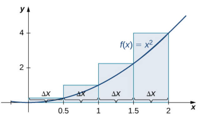
Example: Approximate the area under the curve of $f(x)=x^2$ over $[0,2]$ by partitioning $[0,2]$ into $4$ sub-intervals and using a left-hand-endpoint sum and a right-hand-endpoint sum.
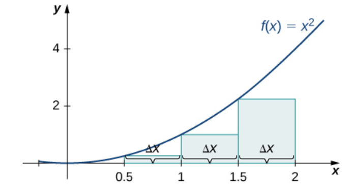
$$L_4=f(x_1^*)\Delta x +f(x_2^*)\Delta x +f(x_3^*)\Delta x+f(x_4^*)\Delta x=\left(\frac{0}{2}\right)^2\frac{1}{2}+\left(\frac{1}{2}\right)^2\frac{1}{2}+\left(\frac{2}{2}\right)^2\frac{1}{2}+\left(\frac{3}{2}\right)^2\frac{1}{2}$$
$$R_4=f(x_1^*)\Delta x +f(x_2^*)\Delta x +f(x_3^*)\Delta x+f(x_4^*)\Delta x=\left(\frac{1}{2}\right)^2\frac{1}{2}+\left(\frac{2}{2}\right)^2\frac{1}{2}+\left(\frac{3}{2}\right)^2\frac{1}{2}+\left(\frac{4}{2}\right)^2\frac{1}{2}$$
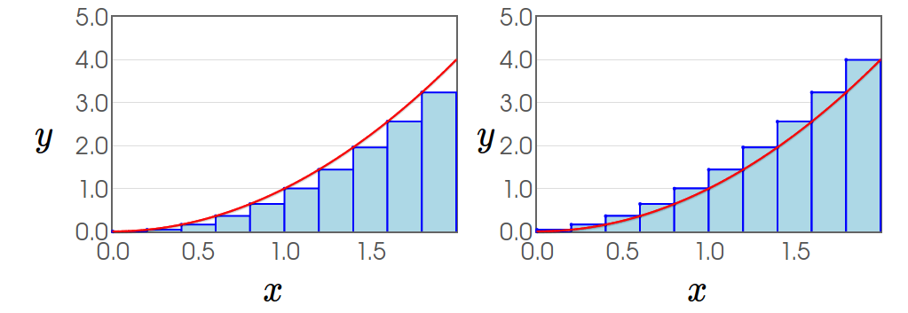
Question: Suppose we want a better approximation. How do we get it?
Another Question: Suppose we want a better approximation with $10$ rectangles. How are we going to write the sum?
Sigma Notation Basics
$$\sum_{i=1}^{n}a_i$$ is a short-hand notation for $$a_1+a_2+a_3+\cdots+a_{n-2}+a_{n-1}+a_n$$
Example: $$\sum_{i=1}^{10}a_i$$ is a short-hand notation for $$a_1+a_2+a_3+a_4+a_5+a_6+a_7+a_8+a_9+a_{10}.$$
Note: the name of the indexing variable is arbitrary. You can all it anything you want. For example, $$\sum_{i=1}^{10}a_i, \,\,\,\, \sum_{j=1}^{10}a_j, \,\,\,\, \sum_{k=1}^{10}a_k, \,\,\,\, \sum_{\Phi=1}^{10}a_\Phi, \,\,\,\, \sum_{\Omega=1}^{10}a_\Omega$$ all represent the same sum $$a_1+a_2+a_3+a_4+a_5+a_6+a_7+a_8+a_9+a_{10}.$$
Example: Setting $a_i=\left(\frac{i}{5}\right)^2\frac{1}{5},$ we can write the left-hand sum $$\scriptsize{L_{10}=\left(\frac{0}{5}\right)^2\frac{1}{5}+\left(\frac{1}{5}\right)^2\frac{1}{5}+\left(\frac{2}{5}\right)^2\frac{1}{5}+\left(\frac{3}{5}\right)^2\frac{1}{5}+\left(\frac{4}{5}\right)^2\frac{1}{5}+\left(\frac{5}{5}\right)^2\frac{1}{5}+\left(\frac{6}{5}\right)^2\frac{1}{5}+\left(\frac{7}{5}\right)^2\frac{1}{5}+\left(\frac{8}{5}\right)^2\frac{1}{5}+\left(\frac{9}{5}\right)^2\frac{1}{5}}$$ as $\scriptsize{L_{10}=\displaystyle \sum_{i=0}^{9}a_i=\displaystyle \sum_{i=0}^{9}\left(\frac{i}{5}\right)^2\frac{1}{5}}.$
Setting $b_i=\left(\frac{i}{5}\right)^2\frac{1}{5},$ we can write the right-hand sum $$\scriptsize{R_{10}=\left(\frac{1}{5}\right)^2\frac{1}{5}+\left(\frac{2}{5}\right)^2\frac{1}{5}+\left(\frac{3}{5}\right)^2\frac{1}{5}+\left(\frac{4}{5}\right)^2\frac{1}{5}+\left(\frac{5}{5}\right)^2\frac{1}{5}+\left(\frac{6}{5}\right)^2\frac{1}{5}+\left(\frac{7}{5}\right)^2\frac{1}{5}+\left(\frac{8}{5}\right)^2\frac{1}{5}+\left(\frac{9}{5}\right)^2\frac{1}{5}+\left(\frac{10}{5}\right)^2\frac{1}{5}}$$ as $\scriptsize{R_{10}=\displaystyle \sum_{i=1}^{10}b_i=\displaystyle \sum_{i=1}^{10}\left(\frac{i}{5}\right)^2\frac{1}{5}}.$
Example: Approximate the area under the curve of $f(x)=x^2$ over $[0,2]$ by partitioning $[0,2]$ into 10 sub-intervals and using a left-hand-endpoint sum and a right-hand-endpoint sum.

$L_{10}=\displaystyle \sum_{i=0}^{9}f(x_i^*)\Delta x=\sum_{i=0}^{9}\left(i\Delta x \right)^2\Delta x= \sum_{i=0}^{9}\left(\frac{i}{5}\right)^2\frac{1}{5}$
$R_{10}=\displaystyle \sum_{i=1}^{10}f(x_i^*)\Delta x=\sum_{i=1}^{10}\left(i \Delta x \right)^2\Delta x=\sum_{i=1}^{10}\left(\frac{i}{5}\right)^2\frac{1}{5}.$
Sigma Notation Basics: Basic Properties
$$\sum_{i=1}^{n}(a_i+b_i)=\sum_{i=1}^{n}a_i+\sum_{i=1}^{n}b_i$$ $$\sum_{i=1}^{n}(a_i-b_i)=\sum_{i=1}^{n}a_i-\sum_{i=1}^{n}b_i$$ $$\sum_{i=1}^{n} k a_i=k\sum_{i=1}^{n}a_i$$
Story Time!
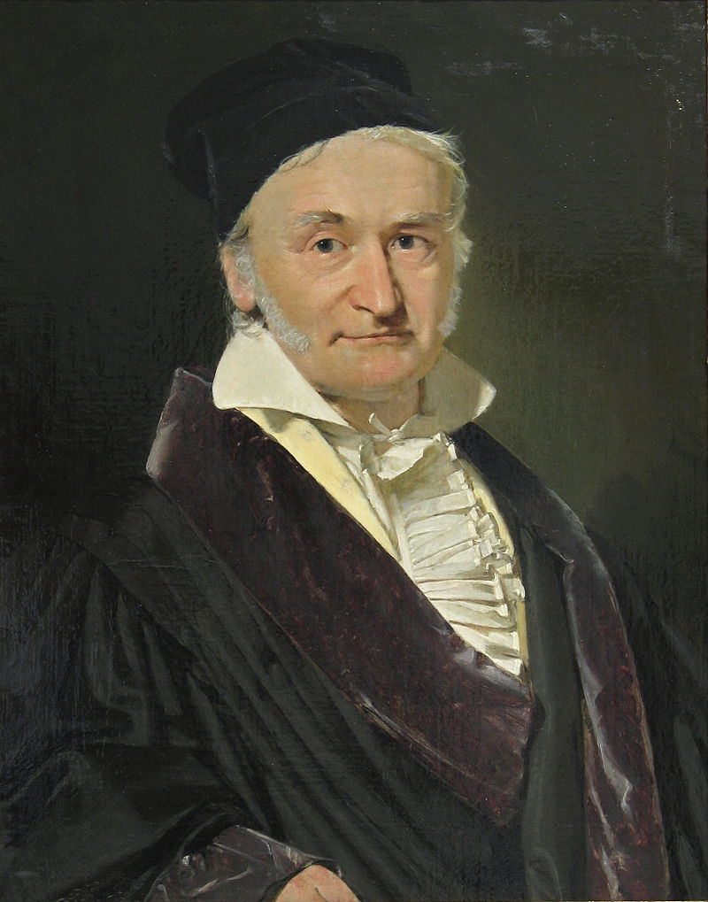
Carl Friedrich Gauss
Some Useful Sums
$$\sum_{i=1}^{n}i=1+2+3+\cdots+n=\frac{n(n+1)}{2}$$ $$\sum_{i=1}^{n}i^2=1^2+2^2+3^2+\cdots+n^2=\frac{n(n+1)(2n+1)}{6}$$ $$\sum_{i=1}^{n}i^3=1^3+2^3+3^3+\cdots+n^3=\left(\frac{n(n+1)}{2}\right)^2$$
Definition: Area Under a Curve
The area under the curve is defined to be the limit of a Riemann Sum: $$\lim_{n \rightarrow \infty} \sum_{i=1}^{n}f(x_i^*)\Delta x$$
Definition: Area Under a Curve
The area under the curve is defined to be the limit of a Riemann Sum: $$\lim_{n \rightarrow \infty} \sum_{i=1}^{n}f(x_i^*)\Delta x$$ We may also choose $x_i^*$ to be the left and right-hand endpoints: $$\lim_{n \rightarrow \infty} \sum_{i=0}^{n-1}f(a+i\Delta x)\Delta x \,\,\,\, \mbox{ and }\,\,\,\, \lim_{n \rightarrow \infty} \sum_{i=1}^{n}f(a+i\Delta x)\Delta x$$ Note that $\displaystyle \Delta x=\frac{b-a}{n},$ where $[a,b]$ is the interval over which we are finding the area.
Definition: Area Under a Curve
The area under the curve is defined to be the limit of a Riemann Sum: $$\lim_{n \rightarrow \infty} \sum_{i=1}^{n}f(x_i^*)\Delta x=\lim_{n \rightarrow \infty} \sum_{i=0}^{n-1}f(i\Delta x)\Delta x=\lim_{n \rightarrow \infty} \sum_{i=1}^{n}f(i\Delta x)\Delta x$$
$y=x^2, \,\, 0 \leq x \leq 2$
| $y$ | $y$ | ||
| $x$ | $x$ |
Example: Find the exact area under the curve of $f(x)=x^2$ over the interval $[0,2]$ as the limit of a Riemann sum.
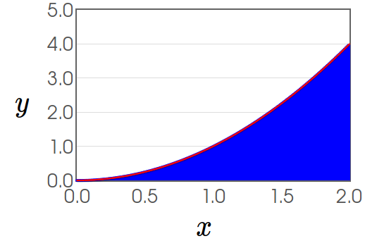
We first find an expression for the area of an approximation using $n$ rectangles.
To do so, we will evaluate a right-hand Riemann sum for with $n$ terms:
$$
\begin{array}{lll}
\displaystyle \sum_{i=1}^{n}f(x_i^*)\Delta x&=\displaystyle \displaystyle \sum_{i=1}^{n}f(a+i\Delta x)\Delta x &\mbox{}\\
&=\displaystyle \sum_{i=1}^{n}f(i\Delta x)\Delta x&\mbox{since $a=0$}\\
&=\displaystyle \sum_{i=1}^{n}(i\Delta x)^2\Delta x&\mbox{since $f(x)=x^2$}\\
&=\displaystyle \sum_{i=1}^{n}\left(\frac{2i}{n}\right)^2\frac{2}{n}&\mbox{since $\displaystyle \Delta x =\frac{b-a}{n}=\frac{2-0}{n}=\frac{2}{n}$}\\
&=\displaystyle \sum_{i=1}^{n}\left(\frac{4i^2}{n^2}\right)\frac{2}{n}&\mbox{}\\
&=\displaystyle \sum_{i=1}^{n}\frac{8i^2}{n^3}&\mbox{}\\
&=\displaystyle \frac{8}{n^3}\sum_{i=1}^{n}i^2&\mbox{since $\displaystyle \sum_{i=1}^{n} k a_i=k\sum_{i=1}^{n}a_i$}\\
\end{array}
$$
We now recall one of our useful sums, $\displaystyle \sum_{i=1}^{n}i^2=1^2+2^2+3^2+\cdots+n^2=\frac{n(n+1)(2n+1)}{6}.$
Then, $$ \begin{array}{lll} \displaystyle \sum_{i=1}^{n}f(x_i^*)\Delta x&=\displaystyle \frac{8}{n^3}\sum_{i=1}^{n}i^2&\mbox{}\\ &\displaystyle =\frac{8}{n^3}\frac{n(n+1)(2n+1)}{6}&\mbox{}\\ &\displaystyle =\frac{8}{n^3}\frac{2n^3+3n^2+n}{6}&\mbox{}\\ &\displaystyle =\frac{16n^3+24n^2+8n}{6n^3}&\mbox{}\\ &\displaystyle =\frac{8}{3}+\frac{4}{n}+\frac{4}{3n^2}&\mbox{}\\ \end{array} $$ Thus the exact area under the curve is $$ \lim_{n \rightarrow \infty}\sum_{i=1}^{n}f(x_i^*)\Delta x =\lim_{n \rightarrow \infty} \left(\frac{8}{3}+\frac{4}{n}+\frac{4}{3n^2}\right) =\frac{8}{3}. $$
Then, $$ \begin{array}{lll} \displaystyle \sum_{i=1}^{n}f(x_i^*)\Delta x&=\displaystyle \frac{8}{n^3}\sum_{i=1}^{n}i^2&\mbox{}\\ &\displaystyle =\frac{8}{n^3}\frac{n(n+1)(2n+1)}{6}&\mbox{}\\ &\displaystyle =\frac{8}{n^3}\frac{2n^3+3n^2+n}{6}&\mbox{}\\ &\displaystyle =\frac{16n^3+24n^2+8n}{6n^3}&\mbox{}\\ &\displaystyle =\frac{8}{3}+\frac{4}{n}+\frac{4}{3n^2}&\mbox{}\\ \end{array} $$ Thus the exact area under the curve is $$ \lim_{n \rightarrow \infty}\sum_{i=1}^{n}f(x_i^*)\Delta x =\lim_{n \rightarrow \infty} \left(\frac{8}{3}+\frac{4}{n}+\frac{4}{3n^2}\right) =\frac{8}{3}. $$
Recall: Lest we get too lost in the clouds, let's not forget that areas under curves are meaningful!
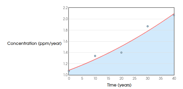
Example: The following table gives approximate values of the average annual atmospheric rate of increase in carbon dioxide ($\mbox{CO}_2$) each decade since $1960,$ in parts per million (ppm). Estimate the total increase in atmospheric $\mbox{CO}_2$ between $1964$ and $2003.$
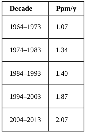
Let's look at a graph of the data:
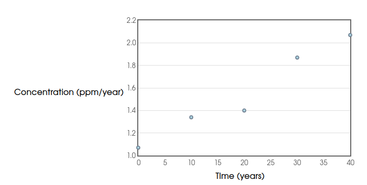
We can estimate the total change by estimating the area under the curve which describes how $\mbox{CO}_2$ concentration varies with time:
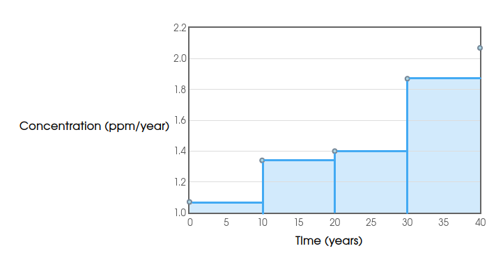
From the above picture, we have a left-hand sum: $$ \begin{array}{ll} \mbox{Total Increase} \approx L_4=\displaystyle \sum_{i=1}^{4}f(x_i^*)\Delta x & = 1.07 \cdot 10 + 1.34 \cdot 10 + 1.40 \cdot 10 + 1.87 \cdot 10 \\ & =10.7+13.4+14.0+18.7\\ & = 56.8 \mbox{ ppm} \end{array} $$ We can also look at the right-hand sum:
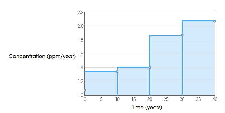
From the above picture: $$ \begin{array}{ll} \mbox{Total Increase} \approx R_4=\displaystyle \sum_{i=1}^{4}f(x_i^*)\Delta x & = 1.34 \cdot 10 + 1.40 \cdot 10 + 1.87 \cdot 10 +2.07 \cdot 10\\ & =13.4+14.0+18.7+20.7\\ & = 66.8 \mbox{ ppm} \end{array} $$ Taking the avarage of these sums gives us a better estimate of the total change in $\mbox{CO}_2$ concentration: $$ \mbox{Total Increase} \approx \frac{L_4+R_4}{2}=\frac{56.8+66.8}{2}=61.8 \mbox{ ppm} $$
Another option is to fit a curve to the data and look at the area under the curve:
 The area under the curve is $61.6507 \mbox{ ppm}$ which is close to our Riemann sum estimate.

We can estimate the total change by estimating the area under the curve which describes how $\mbox{CO}_2$ concentration varies with time:

From the above picture, we have a left-hand sum: $$ \begin{array}{ll} \mbox{Total Increase} \approx L_4=\displaystyle \sum_{i=1}^{4}f(x_i^*)\Delta x & = 1.07 \cdot 10 + 1.34 \cdot 10 + 1.40 \cdot 10 + 1.87 \cdot 10 \\ & =10.7+13.4+14.0+18.7\\ & = 56.8 \mbox{ ppm} \end{array} $$ We can also look at the right-hand sum:

From the above picture: $$ \begin{array}{ll} \mbox{Total Increase} \approx R_4=\displaystyle \sum_{i=1}^{4}f(x_i^*)\Delta x & = 1.34 \cdot 10 + 1.40 \cdot 10 + 1.87 \cdot 10 +2.07 \cdot 10\\ & =13.4+14.0+18.7+20.7\\ & = 66.8 \mbox{ ppm} \end{array} $$ Taking the avarage of these sums gives us a better estimate of the total change in $\mbox{CO}_2$ concentration: $$ \mbox{Total Increase} \approx \frac{L_4+R_4}{2}=\frac{56.8+66.8}{2}=61.8 \mbox{ ppm} $$
Another option is to fit a curve to the data and look at the area under the curve:
