Today we review some basic, prototype categories of functions which we will commonly encounter in this course.
The classes we consider today are
- Linear Functions
- Polynomial Functions
- Piecewise-Defined Functions
Linear Functions
Linear functions can always be written in the form $f(x)=mx+b$ where $m$ is the slope and $b$ is the $y$-coordinate of the $y$-intercept.
Fact: To find the equation of a line, or to graph a line, we need two pieces of information which consist of either:
- A Point and a Slope, or
- Two points.
Example: Use the graph to determine the equation of the line.
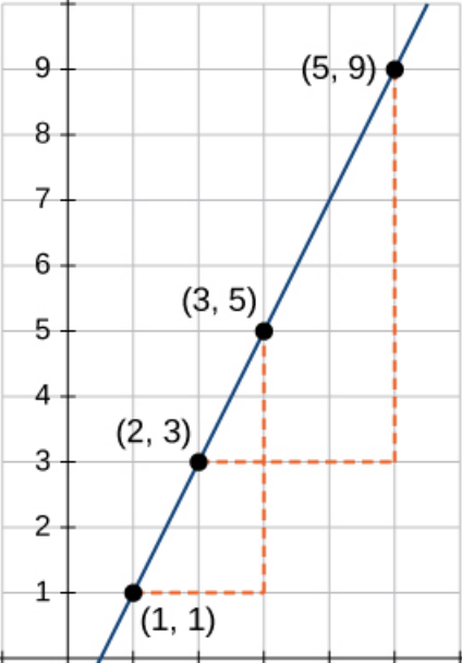
Note: The choice of points we use to determine slope is irrelevant; we will always get the same value.
Another Fun Form: The point slope form. $$y-y_1=m(x-x_1)$$ Example: Write the equation of the line below in point-slope form.
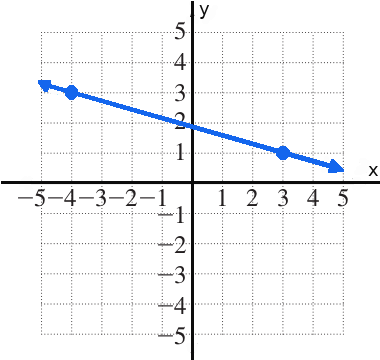
Note: We will make fairly extensive use of this form later on.
The Importance of Slope
Big Fact: The concept of slope will play a central role in this course.
Your understanding of slope as the rate at which the output of a function is changing with respect to the input is vitally important for being able to apply calculus concepts to other topics such as physics, chemistry, and biology. (...among many others!)
Example: The graph gives the distance an automobile has travelled after different periods of time. Determine the slope of this line, and then interpret the meaning of this rate of change.
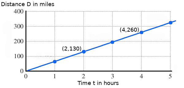
Important Note: In general, the interpretation of slope is $\frac{\mbox{vertical units}}{\mbox{horizontal units}}$.
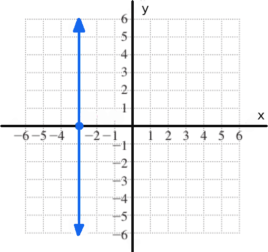
Note: Non-vertical lines are functions. On the other hand, vertical lines are not functions and have an undefined slope. These have the form $x=c$ where $c$ is a constant.
Example: Find the equation of the line below.
Polynomial Functions
Polynomial functions have the form $f(x)=a_n x^n+a_{n-1}x^{n-1}+\cdots+a_2 x^2+a_1 x+a_0.$
Special cases of polynomial functions are:
- Linear Functions (degree $1$): $f(x)=mx+b$
- Quadratic Functions (degree $2$): $f(x)=ax^2+bx+c$
- Cubic Functions (degree $3$): $f(x)=ax^3+bx^2+cx+d$
- Power Functions (degree $n$): $f(x)=ax^n$
Graphing Polynomial Functions: To sketch a basic graph of a polynomial function $f(x)$:
- Determine the end behavior of $f(x)$ by understanding the behavior using the highest-degree term.
- Determine the zeros, or roots, of $f(x).$
- Determine the $y$-intercept.

Mathematical Models
Polynomials are really pliable models for modelling trends, particularly with data.
Example: The graph below gives data for the average rent for a two bedroom domicile in San Francisco since January $2011.$
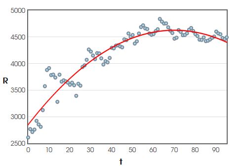
1. What was the approximate average rent during month $25?$
$R({\bf 25})=-0.3625\cdot {\bf 25}^2+50.7599\cdot {\bf 25}+2850.3062 \approx 3892.74$
That is, during month $25$ rent was approximately $\$3892.74$ per month on average.
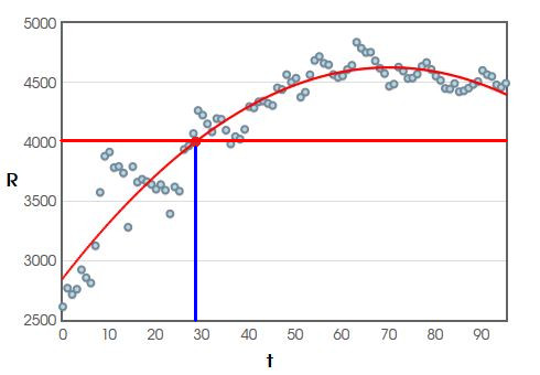
2. In approximately which month did the average rent reach $\$4000?$
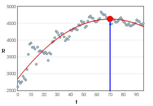
3. In approximately which month did the average rent reach its maximum for the period considered here.
For $R(t)=-0.3625t^2+50.7599t+2850.3062,$ $$t_{max}=\frac{-b}{2a}=\frac{-50.7599}{2\cdot(-0.3625)} \approx 70.01$$ That is, over this period, the average rent reached its maximum in month $70.$
4. Approximately what was the maximum average rent?
For month $70,$ $$R({\bf 70})=-0.3625\cdot {\bf 70}^2+50.7599\cdot {\bf 70}+2850.3062 \approx 4627.25$$ That is, the maximum rent over this period was about $\$4627.25$

Piecewise Defined Functions
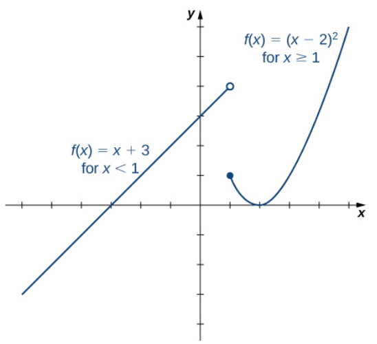
Sometimes we need to define functions in pieces to describe as function such as the one graphed below.
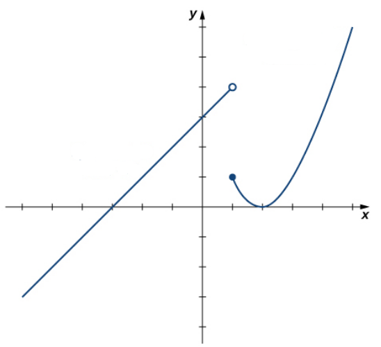
Example: Write a piecewise definition of the above function.
Example: For the piecewise function $$ f(x)= \begin{cases} 4x+3, & x \leq 0 \\ -x+1, & x \gt 0 \end{cases} $$ a. find $f(-3),$ $f(0),$ and $f(2),$ and
b. sketch the graph.

A List of Familiar Prototype Functions We Know... or Should Know $$\displaystyle \begin{array}{lrr} \mbox{Equation} & \mbox{Prototype} & \mbox{Domain}\\ f(x)=c & \mbox{constant} & (-\infty,\infty)\\ f(x)=x & \mbox{identity} & (-\infty,\infty)\\ f(x)=x^2 &\mbox{squaring} & (-\infty,\infty)\\ f(x)=x^3 &\mbox{cubing} & (-\infty,\infty)\\ f(x)=x^n &\mbox{power} & (-\infty,\infty)\\ f(x)=\sqrt{x} &\mbox{square root} & [0,\infty)\\ f(x)=\sqrt[3]{x} &\mbox{cube root} & (-\infty,\infty)\\ f(x)=\sqrt[4]{x} &\mbox{quartic root} & [0,\infty)\\ %f(x)=\sqrt[5]{x} &\mbox{quintic root} & (-\infty,\infty)\\ f(x)=|x| &\mbox{absolute value} & \mathbb{R}=(-\infty,\infty)\\ f(x)=\displaystyle \frac{1}{x} &\mbox{reciprocal} & (-\infty,0)\cup(0,\infty)\\ %f(x)=b^x &\mbox{exponential}\\ %f(x)=\log_b(x) &\mbox{logarithmic}\\ \end{array}$$
Recall: Transformations of prototype functions.
By knowing the graphs of each of these prototype functions, we can graph many functions that are basic transformations of prototype functions.
Also, we can sometimes recognize a graph as a transformed prototype function in order to write its equation.
Example: Vertical Transformations. Prototype function: $$f(x)=x^2$$
Example: Horizontal Transformations. Prototype function: $$f(x)=x^2$$
Generally Speaking...
Suppose you have a graph of $y=f(x).$ Then:
1) The graph of $y=f(x)+c$ is the graph of $y=f(x)$ shifted up $c$ units.
2) The graph of $y=f(x)-c$ is the graph of $y=f(x)$ shifted down $c$ units.
3) The graph of $y=f(x+c)$ is the graph of $y=f(x)$ shifted to the left $c$ units.
4) The graph of $y=f(x-c)$ is the graph of $y=f(x)$ shifted to the right $c$ units.
Example: Combining Transformations. Prototype function: $$f(x)=x^2$$
Example : Consider the basic (prototype) function $f(x)=|x|.$ Write the transformation of $y=f(x)$ which gives the graph below.
$$\begin{array}{ll} y&=f(x+1)-2\\ &=|x+1|-2 \end{array}$$
Example: Find the domain and use transformations to graph the function $$f(x)=\sqrt{x+2}+3.$$

Example: Stretching and Shrinking. Prototype function: $$f(x)=x^2$$
Example: Reflections. Prototype function: $$f(x)=x^2$$
Generally Speaking...
Suppose you have a graph of $y=f(x).$ Then:
1) The graph of $y=cf(x)$ stretched $c$ units when $c \gt 1.$
2) The graph of $y=cf(x)$ is the graph of $y=f(x)$ shrunk down (or compressed) by $c$ when $0 \lt c \lt 1$.
3) The graph of $y=-f(x)$ is the graph of $y=f(x)$ reflected over the $x$ axis.
Example: Combining Transformations. Prototype function: $$f(x)=x^2$$
Example : Consider the basic (prototype) function $f(x)=|x|.$ Write the transformation of $y=f(x)$ which gives the graph below.
$$\begin{array}{ll} y&=2f(x-1)+3\\ &=2|x-1|+3 \end{array}$$
Example: Use transformations to graph the function $$f(x)=0.5(x+2)^2+3.$$
