The random variables we have worked with so far have all been discrete.
Today we address the continuous case.
Example
Suppose we randomly sample from the population of women aged $20$ to $29$ and measure their height, and record the data in a histogram.
The Big Idea
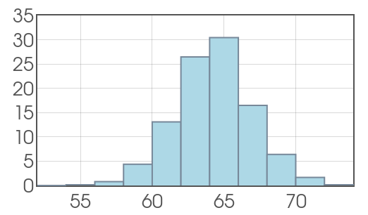
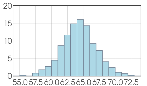
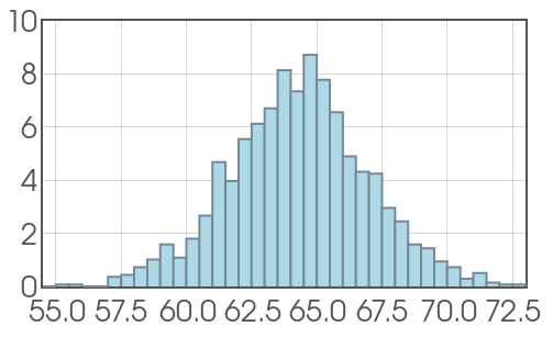
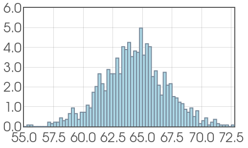
Probability Density Functions

Probability Density Functions
Idea: Suppose we want to estimate the probability that a randomly chosen young woman's height will fall between $68$ and $70$ inches. We could do it using our data.
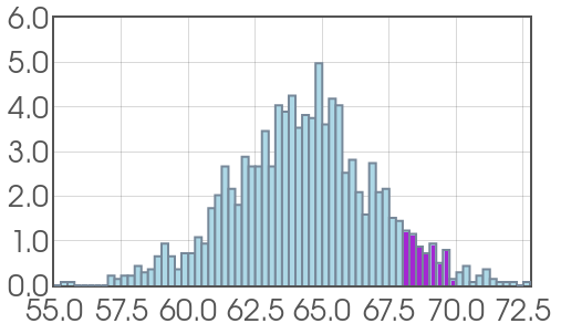
Probability Density Functions
OR we could compute the probability with our probability density function.
 | $\longrightarrow$ | 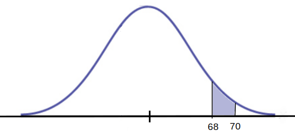 |
PDF Basics
Question: If we added up all the percentages of the bars of our histogram, what percentage should we end up with?

PDF Basics
The total area under any PDF is $1.$ This may be interpreted as $100\%$ of our data is represented by the curve's area.
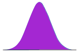
PDF Basics
The PDF curve is represented by a function. We shall often call our PDF $f(x).$
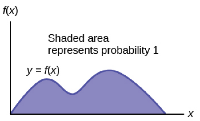
PDF Basics
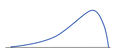
PDFs can take on many different shapes.
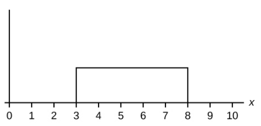
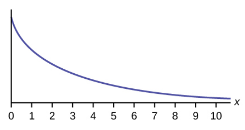
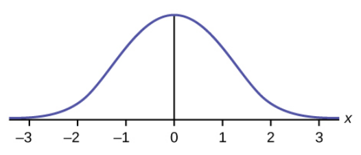
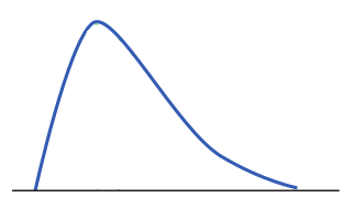
PDF Basics
To compute the probability that a continuous random variable $X$ will take on values between $a$ and $b$ is the area under the curve from $a$ to $b.$
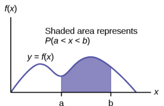
PDF Basics Example: The probability of that a randomly chosen young woman's height is between $68$ and $70$ inches is $0.0679.$

One More Big Idea: The cumulative density function $F(x).$
The cumulative density function (or CDF) gives the probability that a random variable is less than the value $x.$
That is, $F(x)=P(X \lt x),$ and is the area under the PDF up to $x.$
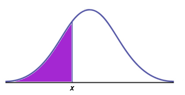
 | $P(X \lt a)=F(a)$ |
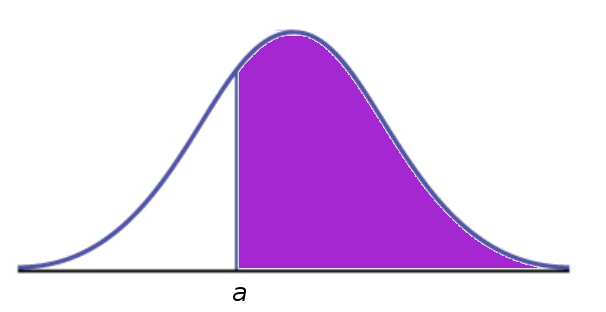 | $P(X \gt a)=1-F(a)$ |
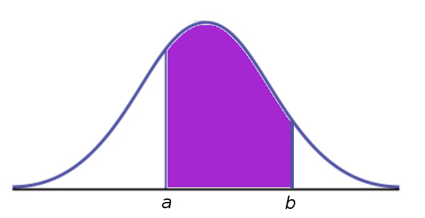 | $P(a \lt X \lt b)=F(b)-F(a)$ |
Do Not Fear!
We will be able to compute areas either by using a formula, a table, or by software.
You will not have to learn any high falutin' methods for finding areas.
An Itty Bitty Detail
Don't let end points stress you out either. Continuous probabilities are the same regardless of whether or not they include the endpoint(s). That is: $$P(X \lt a)=P(X \leq a)$$ $$P(X \gt a)=P(X \geq a)$$ $$P(a \lt X \lt b)=P(a \leq X \lt b)=P(a \lt X \leq b)=P(a \leq X \leq b)$$
An Itty Bitty Detail
This also means (yes, it's counterintuitive) that $P(X=a)=0$ for any continuous random variable $X.$