In calculus, there are two problems that we would like to solve.
1) Find slopes of tangent lines to curves.
2) Find the areas under curves.
Today, we give a sneak preview of the methods we will be using in order to provide motivation for the sections which follow.
What Is a Tangent Line?
Informal Definition: A tangent line to a curve given by a function $y=f(x)$ at the point $x=a$ is a line that intersects the function once near the point $a.$
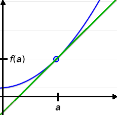
Interpretation: The slope of the tangent line is the slope of the function $y=f(x)$ at the point $x=a.$

How Do we Find the Slope of a Tangent Line?
We shall begin by approximating the slope of the tangent line with the slope of a secant line.
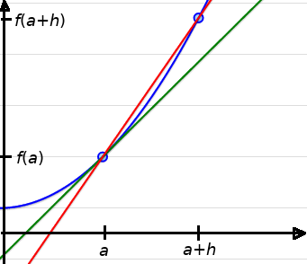
Note: The slopes of the two lines are close to one another.
The Slope of a Secant Line
The slope of the secant line is $\displaystyle \frac{f(a+h)-f(a)}{h}.$
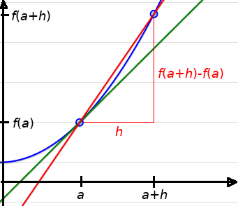
Example: Find the slope of the tangent line to $f(x)=x^2$ at $x=1$ by looking at the behavior of finer approximations using the slope of the secant line.
| $y$ | | |
| $x$ |
Using a Table
To estimate the slope of the tangent line of $f(x)=x^2$ at $x=1,$ we can make a table of values of the slope of the secant line as $h$ gets smaller and our approximation improves.
| $h$ | $\displaystyle \frac{f(1+h)-f(1)}{h}=\frac{(1+h)^2-1}{h}$ |
What is Our Final Conclusion?
We conclude that the slope of the curve $f(x)=x^2$ at $x=1$ is $2.$
Limiting Behavior
We reached our final conclusion by looking at the limiting behavior of the slopes of secants lines in to find the slope of the tangent line.
The number an expression approaches is called the limit of the expression.
In particular, we saw that the expression $\displaystyle \frac{(1+h)^2-1}{h}$ gets closer and closer to $2$ as $h$ gets closer and closer to $0.$
We say that $2$ is the limit of $\displaystyle \frac{(1+h)^2-1}{h}$ as $h$ approaches $0.$
Being able to find slopes of tangent lines is one of many reasons we will be studying limiting behavior in detail in the coming sections.
Big Question: Why would we even want to find the slope of a tangent line?
Big Answer: Because there are tons of useful conclusions we can draw from them!
Slope as a Rate of Change
Recall: To interpret a slope, remember $$\mbox{units of slope}=\frac{\mbox{vertical units}}{\mbox{horizontal units}}$$
Average Rate of Change of a Function
The average rate of change of $f(x)$ over the interval $[a,a+h]$ is $\displaystyle \frac{f(a+h)-f(a)}{h}.$
Instantaneous Rate of Change
The instantaneous rate of change of $f(x)$ at $x=a,$ is the limiting value of the expression $$\displaystyle \frac{f(a+h)-f(a)}{h}$$ as $h$ approaches $0.$
This expression is called the difference quotient.
Rate of Change Example: Velocity
Velocity is the rate at which an object's position changes with respect to time.
Suppose we have a function which gives an object's distance in meters with respect to time in seconds, say $s(t).$
Big Question: What is the meaning of the slope of $s(t)$ at a particular time $t?$
Big Hint: What are its units?
Example: Velocity
The graph gives the distance an automobile has travelled after different periods of time. Determine the slope of this line, and then interpret the meaning of this rate of change.
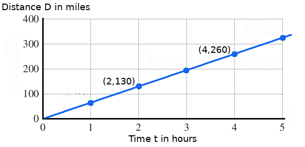
Remember, the interpretation of slope is $\frac{\mbox{vertical units}}{\mbox{horizontal units}}$.
Average Velocity
Suppose we have a function which gives an object's distance in meters with respect to time in seconds, say $s(t).$
The average velocity (in m/sec) of the object over the time interval $[a,a+h]$ is $\displaystyle \frac{s(a+h)-s(a)}{h}.$
Instantaneous Velocity
Suppose we have a function which gives an object's distance in meters with respect to time in seconds, say $s(t).$
The instantaneous velocity at $t=a,$ is the limiting value of the expression $$\displaystyle \frac{s(a+h)-s(a)}{h}$$ as $h$ approaches $0.$
Example: Velocity
Using propane, ethanol, methanol and butane, a potato cannon produce muzzle velocities of between $28$ and $48$ meters per second. (Source: U.S. Air Force Measures Potato Cannon Muzzle Velocities).
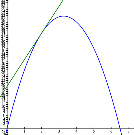
Suppose the muzzle velocity of a potato cannon is $32$ m/s and that the downward acceleration due to gravity is $9.8$ m/s2. Then, when fired vertically, the height $s$ in meters of the potato above the ground $t$ seconds after firing can be expressed (ignoring air resistance) as $s(t)=-4.9t^2+32t.$
What is the velocity of the potato $2$ seconds after firing?
Average Versus Instantaneous Velocity
Consider the equation $s(t)=-4.9t^2+32t$ of the height of our potato with respect to time. The instantaneous velocity of the potato at $t=2$ seconds is $s'(2)=12.4$ m/s
Areas Under Curves
As we mentioned earlier, finding areas under curves is the other big problem calculus seeks to solve.
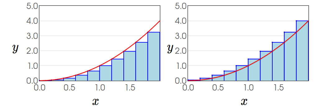
For example, what is the exact area under the curve of the function $f(x)=x^2$ over the interval $[0,2]?$
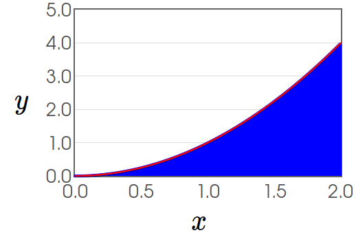
Again, as we shall soon see, the area problem can be reduced to understanding the limiting behavior of certain kinds of expressions.
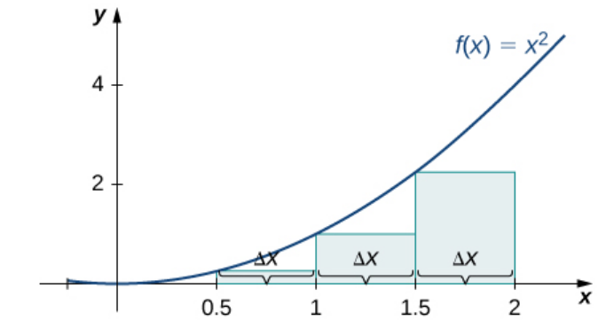
Example: Approximate the area under the curve of $f(x)=x^2$ over $[0,2]$ by partitioning $[0,2]$ into 4 sub-intervals and using a left-hand-endpoint sum and a right-hand-endpoint sum.
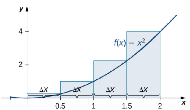
$\mbox{Lower Estimate}=\left(0\right)^2 \cdot 0.5+\left(0.5\right)^2\cdot 0.5+\left(1\right)^2\cdot 0.5+\left(1.5\right)^2\cdot 0.5$
$\mbox{Upper Estimate}=\left(0.5\right)^2 \cdot 0.5+\left(1\right)^2 \cdot 0.5+\left(1.5\right)^2\cdot 0.5+\left(2\right)^2 \cdot 0.5$
Question: Suppose we want a better approximation. How do we get it?
Another Question: Suppose we want a better approximation with $10$ rectangles. How are we going to write the sum?
The Exact Area Under a Curve
In MTH 242, we will find the are under the curve by considering the limit as the width of the rectangles goes to $0:$
$y=x^2, \,\, 0 \leq x \leq 2$
| $y$ | $y$ | ||
| $x$ | $x$ |
Big Question: Why would we even need to find the exact area under a curve?
Big Answer: Because there are tons of useful conclusions we can draw from areas!
For example, if we have a function which describes an object's velocity with respect to time, the area under the curve gives us its change in position!
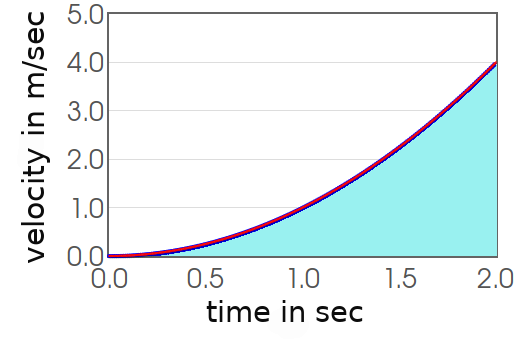 $$\mbox{Units of Area}=\mbox{Horizontal Units} \cdot \mbox{Vertical Units}=\mbox{second} \cdot \frac{\mbox{meters}}{\mbox{second}}=\mbox{meters}$$
One Final Note
It may seem like finding slopes of tangent lines and areas under curve seem like completely unrelated problems.
However, we will learn in MTH 242 that these two problems are intimately related.
For this term, we shall focus on slopes of tangent lines.
The material we shall cover in this next chapter on limiting behavior will set the stage for all that is to come for MTH 241, MTH 242 and beyond!