Polls: When we want to get a sense of how a population feels about an issue, or what candidate they will vote for, we take a poll.
Essentially we want to estimate the percentage, or proportion, of people who will answer in a particular way.
More Generally: when we want to estimate the proportion (i.e., percentage) of observations which fall into a certain category, we use inference for a population proportion.
Other Examples: Estimate the percentage (i.e., proportion) of...
- people who will vote for candidate A
- items in a shipment which are defective
- green M&Ms in a typical pack
- people who smoke
- dead trees killed by drought
- things which fall into some category
Some Big-Time-Super-Important Vocab:
A parameter is a numerical fact about a population. This could be a mean, a standard deviation, a percentage, etc.
A statistic is a value we compute from a sample of our population.
Fact #1: Generally speaking, we don't know the value of a parameter.
Fact #2: We use a statistic to estimate a parameter.
Drawing conclusions about a population from a sample is called inference.
Estimating Parameters: Confidence Intervals
We are now beginning to ride the crest of the statistical wave, folks!
Estimating Parameters: Confidence Intervals
When we estimate a parameter with a sample statistic (in this case, the sample percentage or proportion), we want to know how good our estimate is.
So we construct an interval that captures the true parameter a known percentage the time (i.e, with a known probability).
The interval has the form $$\mbox{estimate} \pm \mbox{margin of error}$$ The details of calculating the margin of error for percentages (proportions) will be one of the focuses of this lecture.
Estimating Proportions
Draw an SRS of size $n$ from a large population that contains proportion $p$ of successes. That is, $100 \cdot p\%$ of the population has some characteristic (i.e. will vote for Candidate A, likes Grumpy Cats Memes, etc.)
Let $\hat{p}$ be the sample proportion (percentage) of successes. Then $$\hat{p}=\frac{\mbox{number of successes}}{\mbox{sample size}}$$ Question: What does the distribution of proportions $\hat{p}$ look like?
Answer
As the sample size increases, the sampling distribution of $\hat{p}$ becomes approximately Normal.
In particular, for large $n$, the sampling distribution of $\hat{p}$ gets closer to $$N\left(p,\sqrt{\frac{p(1-p)}{n}}\right)$$
Recall the 68-95-99.7 Rule
There is an approximately $95\%$ chance that an observation drawn from a normally distributed population will fall within $2$ standard deviations from the mean, in this case $p.$
Since the standard deviation of the $\hat{p}$'s is $\sqrt{\frac{p(1-p)}{n}},$ there is a an approximately $95\%$ chance that $\hat{p}$ will be pinned between the values $p-2\sqrt{\frac{p(1-p)}{n}}$ and $p+2\sqrt{\frac{p(1-p)}{n}}.$ Saying this in pictures...
How to Estimate $p$
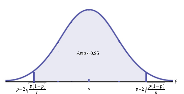
$$P\left(p-2\sqrt{\frac{p(1-p)}{n}} \lt \hat{p} \lt p+2\sqrt{\frac{p(1-p)}{n}}\right) \approx 0.95.$$
How to Estimate $p$
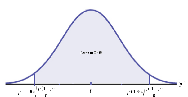
$$P\left(p-1.96\sqrt{\frac{p(1-p)}{n}} \lt \hat{p} \lt p+1.96\sqrt{\frac{p(1-p)}{n}}\right) = 0.95.$$
Performing some algebraic shenanigans on the above, this is equivalent to $$P\left(\hat{p}-1.96\sqrt{\frac{p(1-p)}{n}} \lt p \lt \hat{p}+1.96\sqrt{\frac{p(1-p)}{n}}\right) = 0.95$$ HUGE Question What is the significance of the above probability statement????
Awesome!
So we can just calculate the interval $$ \left( \hat{p}-1.96 \sqrt{\frac{p(1-p)}{n}},\hat{p}+1.96 \sqrt{\frac{p(1-p)}{n}} \right)...$$
...right?
Grumpy Cat Says No... Again

We don't know the true proportion $p,$ so we can't really calculate $\sqrt{\frac{p(1-p)}{n}}$ in the above.
($p$ is the thing we're trying to estimate.)
However...
$\sqrt{\frac{\hat{p}(1-\hat{p})}{n}}$ usually turns out to be a good approximation of $\sqrt{\frac{p(1-p)}{n}}.$

An Approximate 95% Confidence Interval: Interval Notation
Draw an SRS of size $n$ from a large population that contains an unknown proportion $p$ of successes. An approximate $95\%$ confidence interval for $p$ is $$ \left( \hat{p}-1.96 \sqrt{\frac{\hat{p}(1-\hat{p})}{n}},\hat{p}+1.96 \sqrt{\frac{\hat{p}(1-\hat{p})}{n}} \right)$$ Guideline: Use this interval only when the numbers of successes AND failures in the sample are BOTH $15$ or more.
An Approximate 95% Confidence Interval Plus-Or-Minus Notation
Draw an SRS of size $n$ from a large population that contains an unknown proportion $p$ of successes. An approximate $95\%$ confidence interval for $p$ is $$\hat{p} \pm 1.96 \sqrt{\frac{\hat{p}(1-\hat{p})}{n}}$$ Guideline: Use this interval only when the numbers of successes AND failures in the sample are BOTH $15$ or more.
Example: $40\%$ of the dots below are red, and $60\%$ are blue. Let's pretend we don't know this and collect a random sample of dots to estimate the proportion of red dots.
A Kind of Pesky Question: What if we wanted a $99\%$ confidence interval?
A Sort of Nice Answer: We wouldn't have used the value of $1.96$ in our calculation. Instead, we would have used $2.576$.
Why, you ask? Because on a standard normal curve $99\%$ percent of all observations lie between $-2.576$ and $2.576$.
The value of $z$ on the standard normal table which which captures some percentage (i.e., $95\%,$ $99\%,$ etc.) of all values is denoted $z^*$.
A modest table of values of $z^*$: $$ \begin{array}{c|cc} \hline \mbox{Confidence Level $C$} & 90\% & 95\% & 99\%\\ \hline \mbox{Critical Value $z^{*}$} & 1.645 & 1.96 & 2.576 \\ \hline \end{array} $$
An Approximate Confidence Interval: Interval Notation
Draw an SRS of size $n$ from a large population that contains an unknown proportion $p$ of successes. An approximate level $C$ confidence interval for $p$ is $$ \left( \hat{p}-z^* \sqrt{\frac{\hat{p}(1-\hat{p})}{n}},\hat{p}+z^* \sqrt{\frac{\hat{p}(1-\hat{p})}{n}} \right)$$ Guideline: Use this interval only when the numbers of successes AND failures in the sample are BOTH $15$ or more.
An Approximate Confidence Interval Plus-Or-Minus Notation
Draw an SRS of size $n$ from a large population that contains an unknown proportion $p$ of successes. An approximate level $C$ confidence interval for $p$ is $$\hat{p} \pm z^* \sqrt{\frac{\hat{p}(1-\hat{p})}{n}}$$ Guideline: Use this interval only when the numbers of successes AND failures in the sample are BOTH $15$ or more.
Example: From a telephone survey of $229$ Americans, Summer 1994, when asked the question:
"Do you wish Dennis Hopper would go back on drugs?"

$35$ people in the sample answered "yes."
Calculate an approximate $95\%$ confidence interval for the true proportion of Americans who would have answered "yes" to this question.
From the above, we have $k=35$ successes out of $n=229$ observations. This means that there are $194$ failures.
Since the number of successes and failures are BOTH $15$ or more, we may use the large-sample $z$-interval.
We have $\hat{p}=\frac{k}{n}=\frac{35}{229}=0.152$ (to 3 decimal places).
For $95\%$ confidence, we use $z^{*}=1.960.$ Then $$ \begin{array}{ll} &\left( \hat{p}-z^* \sqrt{\frac{\hat{p}(1-\hat{p})}{n}},\hat{p}+z^* \sqrt{\frac{\hat{p}(1-\hat{p})}{n}} \right)\\ =&\left( 0.152-1.960 \sqrt{\frac{0.152 \cdot 0.848}{229}},0.152+1.960 \sqrt{\frac{0.152 \cdot 0.848}{229}} \right)\\ =&(0.105,0.199)\\ =&(10.5\%,19.9\%)\\ \end{array} $$
Problems
One big problem with these techniques is that they give accurate results only when the sample size is large.
Another problem is with small sample sizes, the counts of successes and failures may be too small, rendering the use of these techniques untrustworthy.
Planning a Study: Choosing your sample size.
The margin of error of our large sample confidence interval is $$m=z^*\sqrt{\frac{p(1-p)}{n}}$$ Performing some algebraic shenanigans we get the following nice result...
Planning a Study: Choosing your sample size.
The level $C$ confidence interval for a population proportion $p$ will have margin of error approximately equal to a specified value $m$ when the sample size is $$n=\left(\frac{z^*}{m}\right)^2p^*(1-p^*)$$ where $p^*$ is a guessed value for the sample proportion. The margin of error will always be less than or equal to $m$ if you take the guess $p^*$ to be $0.5.$
Example
The inhabitants of Martiniville, U.S.A. are casting their vote for mayor. On the ballot this election are:
- Sleazy P. Martini (incumbent)
- Stubbs the Cat
Moreover, they all have telephones, they don't lie, and they love to chat on the phone with polsters.
The Situation: We want to estimate the true proportion of Martiniville residents who intend to vote for Stubbs the Cat as mayor within a margin of error of $\pm 3\%$ with $95\%$ confidence. How many people do we need to call?
Another way to ask this is: in repeated samples, how many people would we need to call if we want to get within $3\%$ of the true proportion $95\%$ of the time?
Since we want our margin of error to be $\pm 3\%,$ we take $m=0.03.$
Since our confidence level is $95\%,$ we also have that $z^{*}=1.960.$
We have no idea what $p$ could possibly be, so our guess $p^{*}$ will be $0.5.$ Then, from the formula above we have $$ \begin{array}{ll} n=& \displaystyle \left(\frac{z^*}{m}\right)^2 p^*(1-p^*)\\ =& \displaystyle \left(\frac{1.960}{0.03}\right)^2 (0.5)(0.5)\\ =&1067.\bar{1}\\ \approx & 1068\\ \end{array} $$ Note that we round up so that our margin of error is AT MOST $\pm 3\%.$ Rounding down would mean our margin of error is larger than $\pm 3\%.$
We have no idea what $p$ could possibly be, so our guess $p^{*}$ will be $0.5.$ Then, from the formula above we have $$ \begin{array}{ll} n=& \displaystyle \left(\frac{z^*}{m}\right)^2 p^*(1-p^*)\\ =& \displaystyle \left(\frac{1.960}{0.03}\right)^2 (0.5)(0.5)\\ =&1067.\bar{1}\\ \approx & 1068\\ \end{array} $$ Note that we round up so that our margin of error is AT MOST $\pm 3\%.$ Rounding down would mean our margin of error is larger than $\pm 3\%.$
Let's call a sample of residents in Martiniville to estimate the proportion of people who intend to vote for Stubbs the Cat.
Estimate $\hat{p}$: Margin of Error:
Confidence Interval:
Calling the Election: Who do you think is going to win?