The Normal Distributions

The Normal Distributions Worksheet

Today we learn about one of the most used distributions in all of probability and statistics: the Normal Distribution.

The full truth of this statement will become clearer as we proceed.

Some Places You Might See Normal Distributions

Biology: sizes, heights, weights within a species (from trees to humans). Blood pressure in human adults.

Manufacturing: sizes and weights of mass produced items (diameter sizes of ball bearings, the amount of liquid in a can of soda, the weight of a package of oreos). Measurement errors in all of the above.

Social Sciences: Test scores (IQ, ACT/SAT).

Various: Yearly precipitation in certain parts of the world, the position of a particle that experiences diffusion.

This is all to say that normal distributions are EVERYWHERE!

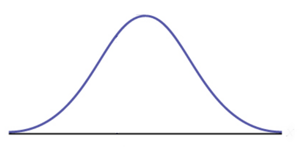
Normal Distribution Basics: The normal distribution is a symmetric, bell-shaped distribution.

Example

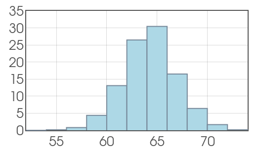
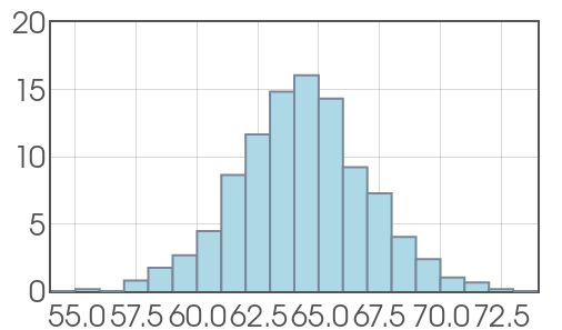
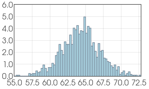
Suppose we randomly sample from the population of women aged $20$ to $29$ and measure their height, and record the data in a histogram.

The Big Idea

Bin Width=

Probability Density Curves

Our histogram can be approximated by a smooth curve. This curve is the probability density curve.

Probability Density Curves

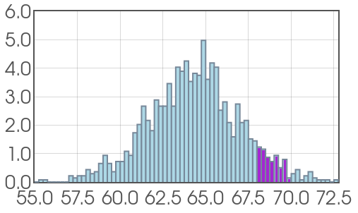
Idea: Suppose we want to estimate the probability that a randomly chosen young woman's height will fall between $68$ and $70$ inches. We could do it using our data.

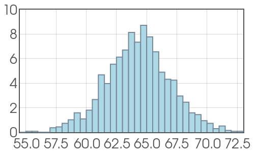
Probability Density Curves

OR we could compute the probability with our probability density curve.

$\longrightarrow$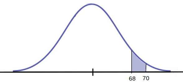

$$\mbox{Probability}=\mbox{Area under the Curve}$$

Density Curve Basics

Question: If we added up all the percentages of the bars of our histogram, what percentage should we end up with?

Density Curve Basics

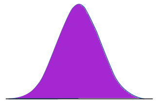
The total area under any Probability Density Curve is $1.$ This may be interpreted as $100\%$ of our data is represented by the curve's area.

$$\mbox{Total Area}=1$$

Normal Distribution Basics

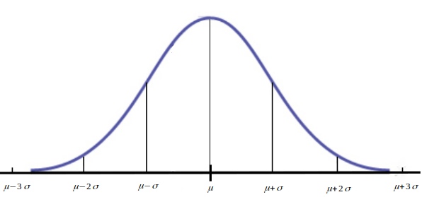
Every normal distribution is determined by two numbers: the mean $\mu$, and the standard deviation $\sigma$.

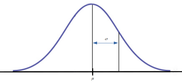
$\mu$ tells us where the center of our distribution is.

$\sigma$ tells us how wide, or "spread out," the distribution is.

Normal Distribution Basics: Examples of Normal Distributions

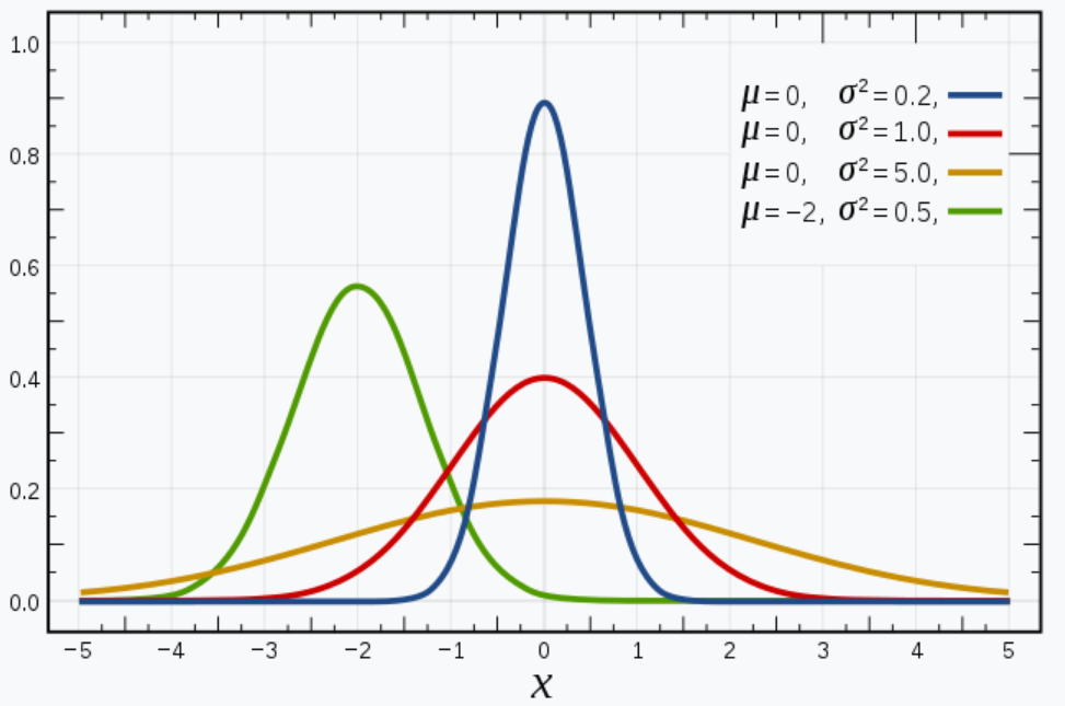
A normal distribution with mean $\mu$ and standard deviation $\sigma$ is denoted as $$N(\mu,\sigma).$$

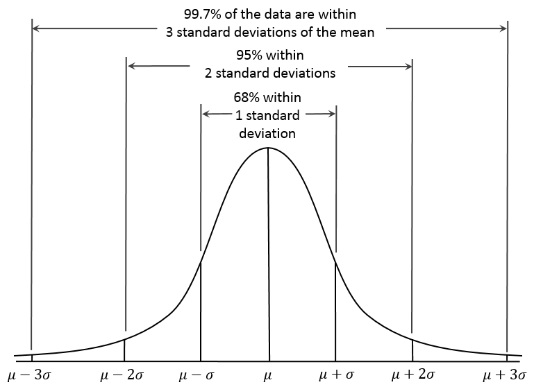
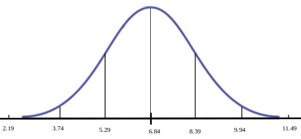
Normal Distribution Basics: The $68\mbox{-}95\mbox{-}99.7$ Rule

For ANY normal distribution:

About $68\%$ of observations lie within $1$ standard deviation of the mean.

About $95\%$ of observations lie within $2$ standard deviations of the mean.

About $99.7\%$ of observations lie within $3$ standard deviations of the mean.

Normal Distribution Basics: The $68\mbox{-}95\mbox{-}99.7$ Rule

Example: Iowa Test Scores. The Iowa Assessments are standardized tests provided as a service to schools by of the University of Iowa.

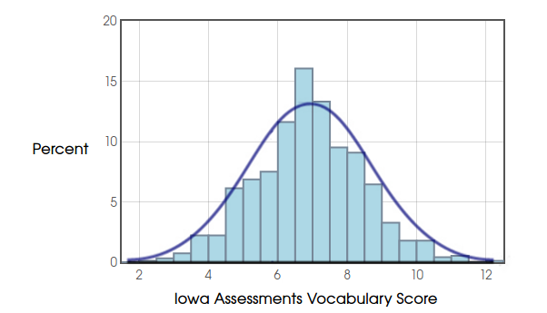
Question: Approximately, what is $\mu$? Approximately, what is $\sigma$?

Example: Iowa Test Scores.

The mean of the Iowa test score data is $6.84,$ and the standard deviation is $1.55.$ The normal distribution $N(6.84,1.55)$ models this data set very well.

Example: Iowa Test Scores & The $68\mbox{-}95\mbox{-}99.7$ Rule

Example: Iowa Test Scores

Question: What percentage of students scored 9 or below?

For a normal distribution $N(\mu, \sigma),$ use the following guide to find the cumulative area:

Compute the value $z=\displaystyle \frac{x-\mu}{\sigma}$ where $x$ is your data point.

Find the value of $z$ in this table.

The number corresponding to this value of $z$ is the cumulative area.

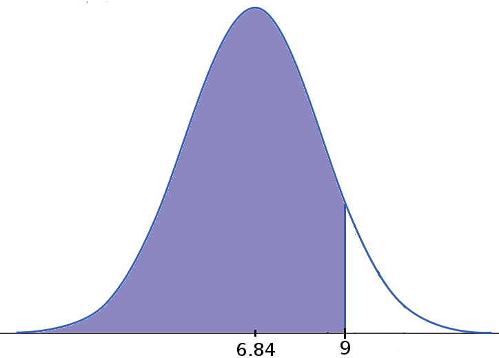
We say that $z$ is the standardized value of $x$. This is also called a $z$-score. It is the number of standard deviations above or below the mean.

Example: Iowa Test Scores. To find $\mbox{Cumulative Area below 9}...$

	$\displaystyle \longrightarrow$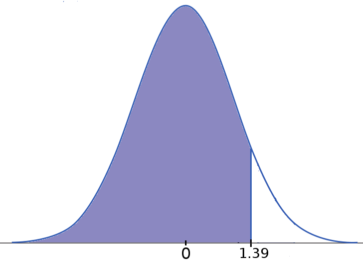
Original: $N(6.84,1.55)$		Standard Normal $N(0,1)$

$$\displaystyle z=\frac{x-\mu}{\sigma}=\frac{9-6.84}{1.55}=1.39$$

Example: Iowa Test Scores.

	$\displaystyle \longrightarrow$
Original: $N(6.84,1.55)$		Standard Normal $N(0,1)$

$$\mbox{Cumulative Area Below 9}=\mbox{Table}(1.39)=0.9177$$

Thus, $91.77\%$ of students scored below $9$ on the Iowa Vocabulary Test.

Put another way, the probability that a randomly chosen student scores $9$ or below is $0.9177.$

Example: Iowa Test Scores

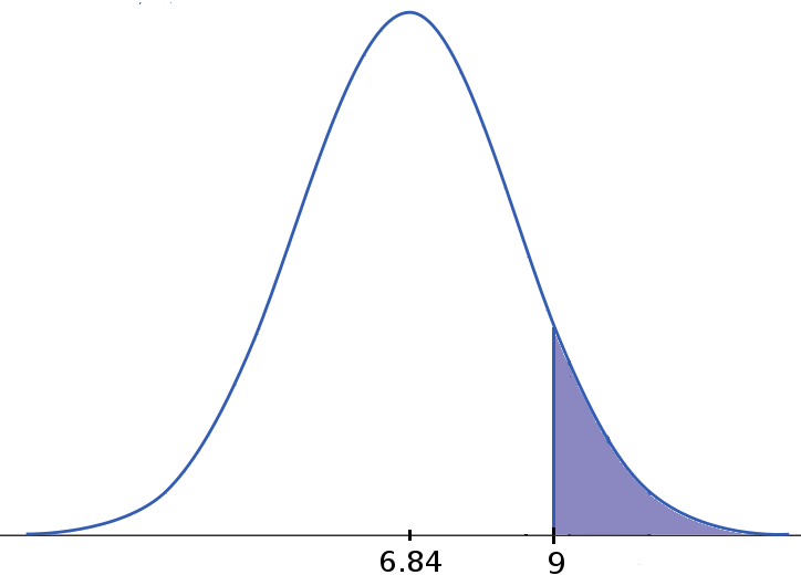
Question: What percentage of students scored above $9?$

$\begin{array}{l} \mbox{Cumulative Area Above 9}\\ =1-\mbox{Cumulative Area Below 9}\\ \approx 1-0.9177\\ = 0.0823 \end{array} $

So about $8.23\%$ of students scored above $9$ on the Iowa Vocabulary Test.

Example: Iowa Test Scores

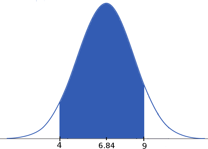
Question: What is the probability a randomly chosen student scored between $4$ and $9?$

Example: Iowa Test Scores.

	$\displaystyle \longrightarrow$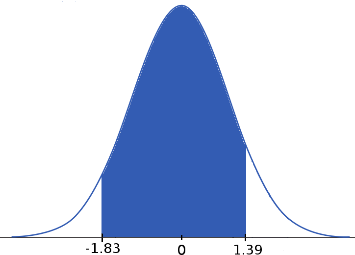
Original: $N(6.84,1.55)$		Standard Normal $N(0,1)$

$\mbox{Area Between 4 and 9}=\mbox{Area Below 9}-\mbox{Area Below 4}$
$=\mbox{Table}(1.39)-\mbox{Table}(-1.83)=0.9177-0.0336=0.8841.$

Interpretation: About $88.41\%$ of students scored between $4$ and $9$ on the Iowa Vocabulary Test.

OR, the probability a randomly chosen student scored between $4$ and $9$ is about $0.8841.$