Question: what are some common statistics you hear about on the news, radio, advertisements, etc.?
Averages
An average is a measure of the center of a distribution. We often call this value the mean and write it as $\overline{x}.$
Example: Find the mean of the data set: $3,$ $3,$ $4,$ $5,$ $7.$
In general, to find the mean of a data set $x_1$, $x_2$, $x_3$,...,$x_n$,
we add up all the observations and divide by the total number of observations.
Using fancy mathematical notation, we write $$ \overline{x}=\frac{x_1+x_2+x_3+\cdots+x_n}{n}=\frac{\displaystyle \sum_\limits{j=1}^{n} x_j}{n} $$
Using fancy mathematical notation, we write $$ \overline{x}=\frac{x_1+x_2+x_3+\cdots+x_n}{n}=\frac{\displaystyle \sum_\limits{j=1}^{n} x_j}{n} $$
Example: Below is a random sample of SAT Critical Reading scores.
$650,$ $490,$ $580,$ $450,$ $570$
Find the the mean, $\overline{x},$ of this data set.
$$
\begin{array}{lll}
\displaystyle \overline{x}&\displaystyle=\frac{\displaystyle \sum_\limits{j=1}^{n} x_j}{n} &\mbox{}\\
\displaystyle &\displaystyle=\frac{x_1+x_2+x_3+\cdots+x_n}{n} &\mbox{}\\
\displaystyle &\displaystyle=\frac{650+490+580+450+570}{5} &\mbox{}\\
\displaystyle &\displaystyle=548 &\mbox{}\\
\end{array}
$$
Calculating the Mean from Grouped Data
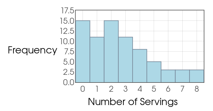
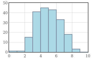
Example: The figure below is a histogram of the number of daily servings of fruit $74$ seventeen-year-old girls claimed to eat. Calculate the mean from this grouped data.
Since we know the frequency of each individual value, we can calculate the mean exactly.
$$ \begin{array}{|l|l|}\hline \mbox{Servings of Fruit} & \mbox{Frequency} \\ \hline \mbox{0} & 15 \\ \hline \mbox{1} & 11 \\ \hline \mbox{2} & 15 \\ \hline \mbox{3} & 11 \\ \hline \mbox{4} & 8 \\ \hline \mbox{5} & 5 \\ \hline \mbox{6} & 3 \\ \hline \mbox{7} & 3 \\ \hline \mbox{8} & 3 \\ \hline \end{array} $$
\begin{array}{rcl}
\bar{x}&=&\displaystyle \frac{\mbox{Total Servings of Fruit}}{\mbox{Number of Girls}}\\
&=&\displaystyle \frac{0 \cdot 15+1 \cdot 11+2 \cdot 15+3 \cdot 11+4 \cdot 8+5 \cdot 5+6 \cdot 3+7 \cdot 3+8 \cdot 3}{15+11+15+11+8+5+3+3+3}\\
&=&\displaystyle \frac{194}{74}\\
&\approx& 2.62
\end{array}
Calculating the Mean from Grouped Data
Note: If given a histogram, we can still calculate the mean.
Estimating Mean from Grouped Data
Example: Below is a frequency table of a random sample of the miles per gallon ratings of 30 cars. Estimate the mean from this grouped data.
Since we DON'T know the frequency of each individual value, we estimate the mean by using the midpoint of each interval instead of actual data values. $$ \begin{array}{|l|l|}\hline\mbox{Mileage} & \mbox{Frequency} \\ \hline \mbox{15 to 20} & 4 \\ \hline \mbox{20 to 25} & 3 \\ \hline \mbox{25 to 30} & 6 \\ \hline \mbox{30 to 35} & 6 \\ \hline \mbox{35 to 40} & 7 \\ \hline \mbox{40 to 45} & 3 \\ \hline \mbox{45 to 50} & 1 \\ \hline\end{array} $$
\begin{array}{rcl}
\bar{x}&=&\displaystyle \frac{\mbox{Sum of Mileages}}{\mbox{Number of Mileages}}\\
&\approx& \displaystyle\frac{17.5 \cdot 4+22.5 \cdot 3+27.5 \cdot 6+32.5 \cdot 6+37.5 \cdot 7+42.5 \cdot 3+47.5 \cdot 1}{4+3+6+6+7+3+1}\\
&=&\displaystyle \frac{935}{30}\\
&\approx& 31.167
\end{array}
Estimating Mean from Grouped Data
Note: If given a histogram, we can still estimate the mean, median, and mode.

Another Measure of Center: The Median. The median is literally the middle value of a data set when we line them all up in order.
Example: Find the median of the data set: $3,$ $3,$ $4,$ $5,$ $7.$
Example: Find the median of the data set: $3,$ $4,$ $5,$ $7.$
Example: Consider a data set of the travel times in minutes for $15$ workers in North Carolina, chosen at random by the Census Bureau which is summarized by the stem plot below. $$ \begin{array}{|r|l|} \hline 0 & 5\\ \hline 1 & 000025\\ \hline 2 & 005\\ \hline 3 & 00\\ \hline 4 & 00\\ \hline 5 & \\ \hline 6 & 0\\ \hline \end{array} $$ What is the median of this data set?
Here's a nice fun thought experiment: Consider the data set
$3,$ $3,$ $4,$ $5,$ $1000000.$
What is the mean of this data set? What is the median?
Example: Suppose the firm "Shady Real-Estate" is advertising a property for sale on Seedy street which is located in a bad area of town. Strangely, an eccentric billionaire has decided to build a house on this street. The following are the prices of the properties on Seedy street:
$\mbox{10,000, 20,000, 35,000, 42,000, 60,000, 10,000,000.}$
What do you think? To entice buyers, Shady Real Estate will report
(a) the mean property value on Seedy street, or
(b) the median property value on Seedy street
Savvy Citizen Fact #1: the mean is very sensitive to extreme observations in data.
The median on the other hand, is not sensitive to extreme observations.
This is why we say that the median is a resistant measure of center.
The mean is therefore NOT a resistant measure of center.
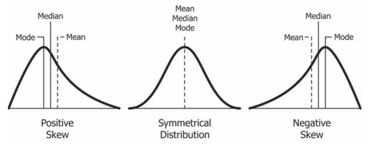
Comparing Means and Medians
The mean and median of a roughly symmetric distribution are close together.
In a skewed distribution, the mean is usually farther out in the long tail than is the median.
Comparing Means, Medians, and Modes
Big Fact: Measures of center aren't enough to adequately describe distributions.
Measures of Center Aren't Enough. To describe a distributions we need more than its center.
Example. Consider the two data sets below:
Data Set 1: $-1,$ $0,$ $1$
Data Set 2: $-1000000,$ $0,$ $1000000$
(a) What are the mean and median of Data Sets $1$ and $2?$
(b) Do the mean and median alone adequately describe these distributions?
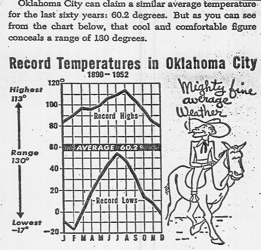
Example: Sleazy P. Martini is a real estate agent for "Shady Real-Estate" and wants to sell you a property for which for which he says "the average yearly temperature is a lovely $60.2$ degrees!"
As a statistically savvy citizen, what questions would you ask Mr. Martini?
Quote of the Day
"A person with their feet in the freezer and their head in the oven is on the average quite comfortable."
Savvy Citizen Fact #2
A useful description of a data set should include not only a measure of center, but also a measure of variation.
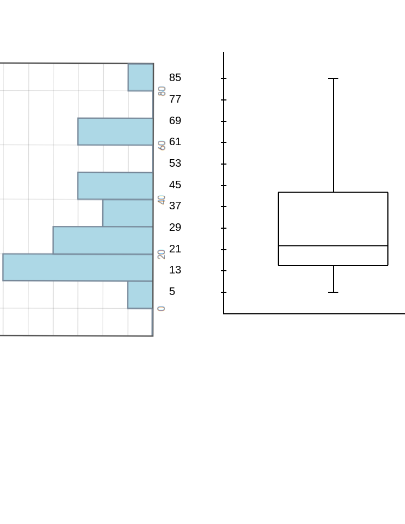
Example. Below are the commute times in minutes of $20$ randomly chosen New York workers.
$10,$ $30,$ $5,$ $25,$ $40,$ $20,$ $10,$ $15,$ $30,$ $20,$ $15,$ $20,$ $85,$ $15,$ $65,$ $15,$ $60,$ $60,$ $40,$ $45$
Arranging these times in ascending order we have
$5,$ $10,$ $10,$ $15,$ $15,$ $15,$ $15,$ $20,$ $20,$ $20$ $|$ $25,$ $30,$ $30,$ $40,$ $40,$ $45,$ $60,$ $60,$ $65,$ $85$
Indicating the medians of the lower 50% and the upper 50% of the data set we have
$5,$ $10,$ $10,$ $15,$ $15,$ $|$ $15,$ $15,$ $20,$ $20,$ $20$ $|$ $25,$ $30,$ $30,$ $40,$ $40,$ $|$ $45,$ $60,$ $60,$ $65,$ $85$
The above gives us a way to describe a distribution with a set of $5$ numbers:
$5,$ $15,$ $22.5,$ $42.5,$ $85$
The numbers
$5,$ $15,$ $22.5,$ $42.5,$ $85$
are a good summary of the New York travel time data as it gives both a measure of the distribution's center and spread.
This collection of numbers actually has a name: the five number summary,
and is in general reported as
$\mbox{Minimum, Quartile 1, Median, Quartile 3, Maximum}$
Of course, you should always plot your data to get a sense of your distribution too! $$ \begin{array}{|r|l|} \hline 0 & 5\\ \hline 1 & 005555\\ \hline 2 & 0005\\ \hline 3 & 00\\ \hline 4 & 005\\ \hline 5 & \\ \hline 6 & 005\\ \hline 7 & \\ \hline 8 & \\ \hline \end{array} $$
Box Plots graphically display the five number summary.
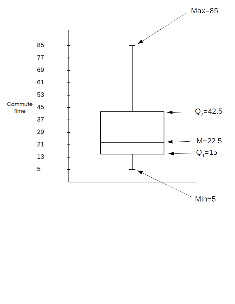
Comparing the box plot of the New York Travel Time data to its stemplot...
Pop Quiz: What is an outlier?
Below is a histogram of our commute-time data. Do you see any potential outliers?
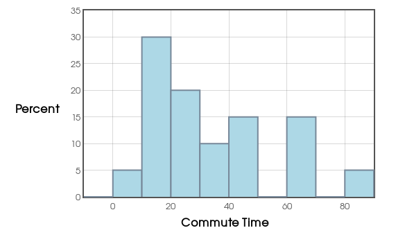
Answer: Yes! The $1.5 \cdot IQR$ rule!
Any data point which strays beyond 1.5 times the $IQR$ is flagged as an outlier.
More Precisely: A value which falls below $Q_1-1.5 \cdot IQR$ or above $Q_3+1.5 \cdot IQR$ is may be considered an outlier.
Example: Does our New York commute-time data contain any outliers according to the $1.5 \cdot IQR$ rule?
$$
\begin{array}{l}
Q_1=15, Q_3=42.5\\
IQR=Q_3-Q_1=42.5-15=27.5\\
\mbox{Lower}=Q_1-1.5 \cdot IQR=15-1.5 \cdot 27.5=-26.25 \\
\mbox{Upper}=Q_3+1.5 \cdot IQR=42.5+1.5 \cdot 27.5=83.75\\
\end{array}
$$
A Numerical Measure of Variation: Standard Deviation
The most common measure of variation is not the quartiles, but the standard deviation.
Standard deviation is like an "average deviation" from the mean.
A Numerical Measure of Variation: Standard Deviation
Example. The standard deviation of the data set $2,$ $2,$ $2$ is $0.$
Example. The standard deviation of the data set $1,$ $2,$ $3$ is $1.$
Example. The standard deviation of the data set $0,$ $2,$ $4$ is $2.$
A Numerical Measure of Variation: Standard Deviation
Each of the data sets below have a a mean $\overline{x}=5.$
How variation from the mean is there in this data set: $5,$ $5,$ $5,$ $5,$ $5,$ $5.$
How variation from the mean is there in this data set: $2,$ $5,$ $4,$ $7,$ $7,$ $5.$
How variation from the mean is there in this data set: $26,$ $-50,$ $4,$ $-40,$ $40,$ $50$
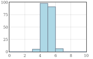
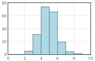
Example: The graphs below have the same mean of $5,$ but increasing standard deviation from left to right.
 |
 |
 |
Standard deviation is a measure of how concentrated a data set is around the mean.
Example: Below is a random sample of SAT Critical Reading scores.
$650,$ $490,$ $580,$ $450,$ $570$
Find the standard deviation of this data set.
The mean is $\overline{x}=548$.
$$ \begin{array}{ccc} \hline \mbox{Data Points} & \mbox{Deviations from the mean} & \mbox{Squared Deviations}\\ \hline 650 & 650 - 548 = 102 & 102^2 = \mbox{10,404} \\ \hline 490 & 490 - 548 = -58 & (-58)^2 = \mbox{3,364} \\ \hline 580 & 580 - 548 = 32 & 32^2 = \mbox{1,024} \\ \hline 450 & 450 - 548 = -98 & (-98)^2 = \mbox{9,604} \\ \hline 570 & 570 - 548 = 22 & 22^2 =484 \\ \hline & \mbox{Sum}=0 & \mbox{Sum=24,880}\\ \end{array} $$
The variance is $\displaystyle \frac{\mbox{24,880}}{4}=6220$.
The standard deviation is: $\sqrt{6220}\approx 78.87$.
Vocab
The variance is the "funny average" of the squared deviations from the mean.
The standard deviation is the square root of the variance.
In general, to find the standard deviation $s$ of a data set:
1) Compute the mean $\overline{x}$.
2) Compute the deviations from the mean.
3) Square all the deviations from the mean.
4) Add up the squared deviations from the mean.
5) Divide the result by $n-1$ (the resulting number is the variance)
6) Take a square root (the resulting number is the standard deviation)
The above steps are summarized by the formula for $s$: $$ s=\sqrt{\frac{(x_1-\overline{x})^2+(x_2-\overline{x})^2+\cdots+(x_n-\overline{x})^2}{n-1}} =\sqrt{\frac{\displaystyle \sum_\limits{j=1}^{n} (x_j-\overline{x})^2}{n-1}} $$
Technology Reminder
$650,$ $490,$ $580,$ $450,$ $570$
Don't forget you may (and should) use your TI-84 Calculator.
And, of course, there's always Holt.Blue.
Fact: A VERY common summary of a distribution is the mean $\overline{x}$ and standard deviation $s$.
Warning: this is only a good idea if your distribution is symmetric!
For skewed distributions it is generally better to use the five number summary: $$\mbox{Min,$Q1,$ Med, $Q3,$ Max}$$